Week 6 — Search and Hashing
CEN207 Data Structures (formerly CE205) · Fall 2026–2027
Lecture notes (PDF) Lecture notes (DOCX) Slides (PDF) Slides (PPTX) Slides (HTML, offline) Download all (ZIP) Open slides full screen
Click inside the slides and use the arrow keys; use the button at the bottom right of the slides, or the "Open slides full screen" link above, for full screen.
This week
Learning outcomes. By the end of this week you will be able to explain, draw, and implement four searching techniques that go beyond the linear and binary search you already know — jump search, interpolation search, exponential search, and Fibonacci search — and you will be able to explain why each one exists (what specific weakness of binary search it fixes, and at what cost). You will then meet an entirely different idea for answering "is x here, and if so, where?": instead of narrowing a range by comparing, a hash table computes the answer's location directly with a hash function, giving average-case O(1) lookup. You will learn the division method h(k) = k mod m and why the choice of m matters; how collisions — two different keys landing on the same slot — are unavoidable and must be resolved, first with separate chaining (a linked list per slot) and then with open addressing (linear probing, quadratic probing, double hashing — every key living inside the table itself); and why a hash table must occasionally rehash — grow and rebuild itself — to keep its performance guarantee as it fills up. These outcomes map to LO.1 (explain fundamental data structures), LO.2 (analyze algorithmic complexity), and LO.7 (choose the right structure for a problem) of the course syllabus.
What you need already. Week 1 gave you arrays and the idea of an index as a direct memory address. Week 2 gave you the linked list — exactly what a hash bucket's chain is built from. Week 3 gave you the stack and the queue. Week 4 gave you trees, and specifically the idea that halving a search space at every step gives you a logarithmic number of steps — that is precisely what binary search already does over an array, and precisely what this week's new searches either exploit further or trade away on purpose. Week 5 gave you graphs and traversal. This week does not build directly on any single one of those data structures; instead it builds on the idea of a sorted array (Week 1) for the four new searches, and introduces the hash table as a genuinely new structure — one that will itself become a useful tool inside later data structures (an adjacency list keyed by a hash map, for instance, when a graph's vertices are not conveniently numbered 0..V-1).
Time plan for a 3-hour session. The search problem, recap of linear and binary search (~15 min) · jump search (~20 min) · interpolation search (~20 min) · exponential search (~15 min) · Fibonacci search (~15 min) · comparison table and a short break · hashing: inception and the division hash function (~20 min) · collisions and separate chaining (~20 min) · open addressing: linear, quadratic, and double hashing (~35 min) · rehashing (~15 min) · choosing a technique, wrap-up and self-check (~15 min).
0. Before we start
0.1 What you already know
Two ideas from the last five weeks matter most this week.
From Week 1 — arrays and indices. An array stores its elements in one contiguous block of memory, and arr[i] is computed directly as base_address + i * element_size — no searching required to reach index i, only to decide which i holds what you want. Every search technique this week (jump, interpolation, exponential, Fibonacci) is a different strategy for choosing which indices to check, on a sorted array, to find that i in as few comparisons as possible. Binary search, already familiar to you, is one point in this design space; this week fills in the rest of it.
From Week 4 — halving a search space. Binary search's big idea — eliminate half the remaining candidates with a single comparison, giving O(log n) total comparisons — is the yardstick every technique in this chapter is measured against. Jump search deliberately does worse than binary search (in exchange for simplicity); interpolation search does better on the right kind of data; exponential search adapts binary search to array sizes you do not know in advance; Fibonacci search matches binary search's asymptotic cost using only addition and subtraction. Keep binary search's O(log n) in your head as the reference point for all four.
A genuinely new idea: trading order for computation. Every technique above still works by comparing target against array elements and narrowing a range. Hashing throws that whole approach away: instead of narrowing, a hash function computes directly where a key belongs, in one O(1) step, with no order requirement on the data at all. The price is that two different keys can compute to the same location — a collision — and the second half of this week is entirely about handling that.
0.2 The map of this week
flowchart TD
    W6["Week 6: Search and Hashing"]
    W6 --> S["Beyond binary search (still comparison-based, still need a SORTED array)"]
    S --> S1["Jump search: fixed-size blocks, O(sqrt n)"]
    S --> S2["Interpolation search: a formula estimates the position"]
    S --> S3["Exponential search: double a bound, then binary search inside it"]
    S --> S4["Fibonacci search: split with Fibonacci numbers, only +/-"]
    W6 --> H["Hashing: compute the location instead of comparing for it"]
    H --> H1["Hash function: h(k) = k mod m (division method)"]
    H --> H2["Collisions are unavoidable -- two keys, one slot"]
    H2 --> C1["Separate chaining: a linked list per slot"]
    H2 --> C2["Open addressing: the key lives IN the table"]
    C2 --> O1["Linear probing: h, h+1, h+2, ... (primary clustering)"]
    C2 --> O2["Quadratic probing: h+1^2, h+2^2, ... (needs m prime, alpha <= 0.5)"]
    C2 --> O3["Double hashing: h1(k), step h2(k) (best spread in practice)"]
    H --> R["Rehashing: grow the table when it fills up, amortized O(1) insert"]
Every box gets its own section below, most with a step-by-step animation, a complete C and Java program, and a note on complexity and common mistakes.
1. The search problem, and a recap of linear and binary search
1.1 The problem, restated
You already solved the basic version of this problem in Week 1: given an array and a target value, is target in the array, and if so, at which index? Week 1 gave you two answers — linear search (check every element, O(n)) and binary search (on a sorted array, repeatedly check the middle and discard half, O(log n)). This week's question is sharper: given that the array is sorted, is binary search's O(log n) really the best we can do, and what does it cost to do better, or to do almost as well with a simpler idea? The four new techniques below each answer that question differently.
1.2 Recap: linear search, O(n)
Linear search makes no assumption about the data at all: it checks arr[0], then arr[1], and so on, until it finds target or runs out of array. Its cost is proportional to n, the array's size, in the worst case (the target is last, or absent) and on average (for a target present at a uniformly random position, you check n/2 elements on average). Its one great virtue is that it works on any array, sorted or not — every technique from here on trades that generality away in exchange for speed, by requiring the array to be sorted first.
1.3 Recap: binary search, O(log n)
Binary search requires a sorted array. It checks the middle element; if it is the target, done; if the target is smaller, the entire right half — including the middle — can be discarded in one step (sorted order guarantees the target cannot be there); if larger, the left half is discarded the same way. Each comparison halves the remaining candidates, so after k comparisons at most n / 2^k candidates remain; the search ends when that reaches 1, giving k = log2(n) comparisons in the worst case — O(log n). For n = 1,000,000, that is about 20 comparisons, versus up to a million for linear search on the same data.
If binary search, its complexity, and its C/Java code are not fresh in your memory, revisit Week 1 before continuing — this chapter assumes it and will not re-derive it. The four techniques below all still require a sorted array, and all are still fundamentally comparison-based; none of them beats binary search's O(log n) worst case by more than a constant factor except interpolation search on the right kind of data (and even that has a bad worst case, as you will see in section 3).
2. Jump search
2.1 A question to start
Binary search's jump to the exact middle is powerful, but it needs a division (or a shift) and a bit of careful index arithmetic (lo + (hi - lo) / 2, to avoid overflow) at every single step, and it does not access memory sequentially — it jumps all over the array, which is unfriendly to hardware that likes to read memory in contiguous blocks (a fact you will meet in more depth when this course reaches memory hierarchies and caching). What if, instead, you scanned forward in fixed-size blocks — check every k-th element, and once you have jumped past where target must be, fall back to a plain linear scan of just that one block? That is jump search: simpler arithmetic than binary search, sequential memory access within each block, at the cost of being asymptotically slower than binary search (though still far faster than linear search).
This block-style search appears in Donald Knuth's The Art of Computer Programming, Volume 3: Sorting and Searching (1973) as an alternative to binary search, presented specifically as a case where a simple calculus argument — minimizing the sum of two costs — determines the algorithm's one free parameter, the block size.
2.2 The idea and the right block size
Pick a block size b. Check arr[b-1], arr[2b-1], arr[3b-1], … until you find a boundary that is >= target (or run off the end of the array); target, if present, must be in the block just before that boundary (sorted order again). Then scan that one block linearly, left to right, comparing every element.
How many comparisons does this cost in the worst case? Jumping costs at most n / b comparisons (you jump through the whole array in blocks of size b), and the final linear scan costs at most b comparisons. Total: n/b + b. Calculus (or just trying values) shows this sum is minimized when b = sqrt(n), giving a total worst-case cost of 2 * sqrt(n) — O(sqrt(n)). That is worse than binary search's O(log n) (for n = 1,000,000, sqrt(n) = 1000 versus log2(n) ≈ 20), but far better than linear search's O(n), and the arithmetic at each step is a single addition, not a division.
2.3 In memory, and the code
Below, jump_search computes block = floor(sqrt(n)), jumps forward one block at a time by checking the last index of each block, and once it finds a block whose last index is >= target, scans that block linearly.
int jump_search(const int arr[], int n, int target, int *comparisons) {
    int block = (int) sqrt((double) n);      /* block size = floor(sqrt(n)) */
    if (block < 1) block = 1;
    int prev = 0, step = block, comp = 0;
    while (step < n) {                        /* jump forward one block at a time */
        comp++;
        if (arr[step - 1] >= target) break;    /* target may be in this block */
        prev = step;
        step += block;
    }
    if (step > n) step = n;
    for (int i = prev; i < step; i++) {        /* linear scan inside the block */
        comp++;
        if (arr[i] == target) { *comparisons = comp; return i; }
        if (arr[i] > target) break;             /* sorted: no need to look further */
    }
    *comparisons = comp;
    return -1;
}
static int jumpSearch(int[] arr, int target) {
    int n = arr.length;
    int block = (int) Math.sqrt(n);          // block size = floor(sqrt(n))
    if (block < 1) block = 1;
    int prev = 0, step = block;
    comparisons = 0;
    while (step < n) {                        // jump forward one block at a time
        comparisons++;
        if (arr[step - 1] >= target) break;    // target may be in this block
        prev = step;
        step += block;
    }
    if (step > n) step = n;
    for (int i = prev; i < step; i++) {        // linear scan inside the block
        comparisons++;
        if (arr[i] == target) return i;
        if (arr[i] > target) break;             // sorted: no need to look further
    }
    return -1;
}
Play the animation to watch the block boundaries get checked one by one, then the final block scanned left to right.
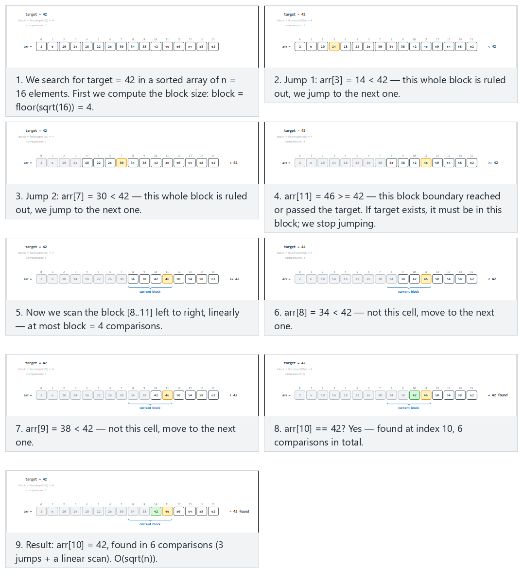
In the picker, also try target near the last block, needs the most jumps (hard) and the edge cases target is smaller than every value, target is larger than every value, and target is in range but not in the array — or press 🎲 for random data at four difficulty levels, or type your own sorted array and target.
2.4 Try it
Full program: jump_search.c / JumpSearch.java
/* Week 6 -- Search and Hashing
 * Jump search: on a SORTED array, jump forward in fixed-size blocks
 * (block = floor(sqrt(n))) until a block boundary is >= target, then scan
 * that block linearly. Prints every jump and every comparison inside the
 * final block.
 * CEN207 Data Structures (formerly CE205)
 */
#include <stdio.h>
#include <math.h>

int jump_search(const int arr[], int n, int target, int *comparisons) {
    int block = (int) sqrt((double) n);      /* block size = floor(sqrt(n)) */
    if (block < 1) block = 1;
    int prev = 0, step = block, comp = 0;
    while (step < n) {                        /* jump forward one block at a time */
        comp++;
        printf("  jump: check arr[%d] = %d\n", step - 1, arr[step - 1]);
        if (arr[step - 1] >= target) break;    /* target may be in this block */
        prev = step;
        step += block;
    }
    if (step > n) step = n;
    printf("  scanning block [%d..%d)\n", prev, step);
    for (int i = prev; i < step; i++) {        /* linear scan inside the block */
        comp++;
        printf("  compare arr[%d] = %d\n", i, arr[i]);
        if (arr[i] == target) { *comparisons = comp; return i; }
        if (arr[i] > target) break;             /* sorted: no need to look further */
    }
    *comparisons = comp;
    return -1;
}

static void print_array(const int arr[], int n) {
    printf("arr =");
    for (int i = 0; i < n; i++) printf(" %d", arr[i]);
    printf("\n");
}

static void run_scenario(const char *label, const int arr[], int n, int target) {
    printf("-- %s --\n", label);
    print_array(arr, n);
    printf("target = %d\n", target);
    int comparisons = 0;
    int index = jump_search(arr, n, target, &comparisons);
    if (index == -1) printf("result: not found, %d comparisons\n\n", comparisons);
    else printf("result: found at index %d, %d comparisons\n\n", index, comparisons);
}

int main(void) {
    int a[] = {2, 6, 10, 14, 18, 22, 26, 30, 34, 38, 42, 46, 50, 54, 58, 62};
    int n = 16;

    run_scenario("normal: 16 values, target found in the second block", a, n, 42);
    run_scenario("hard: target near the last block, needs the most jumps", a, n, 58);
    run_scenario("edge: target is smaller than every value", a, n, 1);
    run_scenario("edge: target is larger than every value", a, n, 999);
    run_scenario("edge: target is in range but not in the array", a, n, 45);

    return 0;
}
/* Week 6 -- Search and Hashing
 * Jump search: on a SORTED array, jump forward in fixed-size blocks
 * (block = floor(sqrt(n))) until a block boundary is >= target, then scan
 * that block linearly. Prints every jump and every comparison inside the
 * final block.
 * CEN207 Data Structures (formerly CE205)
 */
public class JumpSearch {
    static int comparisons;

    static int jumpSearch(int[] arr, int target) {
        int n = arr.length;
        int block = (int) Math.sqrt(n);          // block size = floor(sqrt(n))
        if (block < 1) block = 1;
        int prev = 0, step = block;
        comparisons = 0;
        while (step < n) {                        // jump forward one block at a time
            comparisons++;
            System.out.println("  jump: check arr[" + (step - 1) + "] = " + arr[step - 1]);
            if (arr[step - 1] >= target) break;    // target may be in this block
            prev = step;
            step += block;
        }
        if (step > n) step = n;
        System.out.println("  scanning block [" + prev + ".." + step + ")");
        for (int i = prev; i < step; i++) {        // linear scan inside the block
            comparisons++;
            System.out.println("  compare arr[" + i + "] = " + arr[i]);
            if (arr[i] == target) return i;
            if (arr[i] > target) break;             // sorted: no need to look further
        }
        return -1;
    }

    static void printArray(int[] arr) {
        StringBuilder sb = new StringBuilder("arr =");
        for (int v : arr) sb.append(' ').append(v);
        System.out.println(sb);
    }

    static void runScenario(String label, int[] arr, int target) {
        System.out.println("-- " + label + " --");
        printArray(arr);
        System.out.println("target = " + target);
        int index = jumpSearch(arr, target);
        if (index == -1) System.out.println("result: not found, " + comparisons + " comparisons");
        else System.out.println("result: found at index " + index + ", " + comparisons + " comparisons");
        System.out.println();
    }

    public static void main(String[] args) {
        int[] a = {2, 6, 10, 14, 18, 22, 26, 30, 34, 38, 42, 46, 50, 54, 58, 62};

        runScenario("normal: 16 values, target found in the second block", a, 42);
        runScenario("hard: target near the last block, needs the most jumps", a, 58);
        runScenario("edge: target is smaller than every value", a, 1);
        runScenario("edge: target is larger than every value", a, 999);
        runScenario("edge: target is in range but not in the array", a, 45);
    }
}
Try it
Expected output:
-- normal: 16 values, target found in the second block --
arr = 2 6 10 14 18 22 26 30 34 38 42 46 50 54 58 62
target = 42
  jump: check arr[3] = 14
  jump: check arr[7] = 30
  jump: check arr[11] = 46
  scanning block [8..12)
  compare arr[8] = 34
  compare arr[9] = 38
  compare arr[10] = 42
result: found at index 10, 6 comparisons

-- hard: target near the last block, needs the most jumps --
arr = 2 6 10 14 18 22 26 30 34 38 42 46 50 54 58 62
target = 58
  jump: check arr[3] = 14
  jump: check arr[7] = 30
  jump: check arr[11] = 46
  scanning block [12..16)
  compare arr[12] = 50
  compare arr[13] = 54
  compare arr[14] = 58
result: found at index 14, 6 comparisons

-- edge: target is smaller than every value --
arr = 2 6 10 14 18 22 26 30 34 38 42 46 50 54 58 62
target = 1
  jump: check arr[3] = 14
  scanning block [0..4)
  compare arr[0] = 2
result: not found, 2 comparisons

-- edge: target is larger than every value --
arr = 2 6 10 14 18 22 26 30 34 38 42 46 50 54 58 62
target = 999
  jump: check arr[3] = 14
  jump: check arr[7] = 30
  jump: check arr[11] = 46
  scanning block [12..16)
  compare arr[12] = 50
  compare arr[13] = 54
  compare arr[14] = 58
  compare arr[15] = 62
result: not found, 7 comparisons

-- edge: target is in range but not in the array --
arr = 2 6 10 14 18 22 26 30 34 38 42 46 50 54 58 62
target = 45
  jump: check arr[3] = 14
  jump: check arr[7] = 30
  jump: check arr[11] = 46
  scanning block [8..12)
  compare arr[8] = 34
  compare arr[9] = 38
  compare arr[10] = 42
  compare arr[11] = 46
result: not found, 7 comparisons
2.5 Complexity, mistakes, self-check
Complexity. Best case O(1) (target is the very first block boundary checked and happens to be the target itself — rare, since the boundary check is >=, not ==). Worst case and average case both O(sqrt(n)), with the optimal block size b = sqrt(n) derived in section 2.2. It needs a sorted array, just like binary search.
Common mistakes
- Picking an arbitrary block size (say, a fixed
100) instead of computingsqrt(n). A block size that does not scale withndegrades towardO(n)for large arrays (too many jumps) or toward a large constant scan for small arrays (too much linear work per block); onlyb = sqrt(n)balances the two costs. - Checking
arr[step]instead ofarr[step - 1]. The block boundary you want to test is the last element of the current block (indexstep - 1), not the first element of the next block (indexstep) — off by one here either skips a valid block or scans one element too many. - Forgetting to clamp
steptonafter the jump loop ends. If the last jump overshoots the array (step > n), the linear scan must stop atn, notstep, or it reads past the end of the array.
Self-check: why sqrt(n)?
Jump search costs at most n/b jump-comparisons plus at most b linear-scan comparisons, total n/b + b. Why does calculus say b = sqrt(n) minimizes this sum, and what would happen to the total cost if you instead picked b = 1 or b = n?
Answer. Minimizing f(b) = n/b + b: take the derivative, f'(b) = -n/b^2 + 1, set it to zero: b^2 = n, so b = sqrt(n). At b = 1, jump search degenerates into linear search (n jump-comparisons, each block is one element) — O(n). At b = n, there is only one giant "block" (the whole array), so it degenerates into an ordinary linear scan too — O(n). Only b = sqrt(n) gives the balanced O(sqrt(n)).
3. Interpolation search
3.1 A question to start
Think about how you look up a name in a paper phone book (or a word in a printed dictionary). You do not open it exactly in the middle every time, the way binary search would. If you are looking for "Yilmaz", you open the book much closer to the end; if you are looking for "Aydin", much closer to the start. You are using the fact that names are not just sorted, but roughly uniformly spread out across the alphabet, to jump straight to a good estimate of the right page. Interpolation search does exactly this on a sorted array of numbers: instead of always checking the middle, it computes an estimated position with a formula, using how far target sits between the smallest and largest values currently in range.
This position-estimating idea for searching ordered data appears in W. W. Peterson's 1957 paper Addressing for Random-Access Storage (IBM Journal of Research and Development) — the same early paper that laid out foundational ideas for organizing random-access storage that this week's later sections on hashing also draw on — and was subsequently formalized and analyzed under the name interpolation search.
3.2 The formula
Within the current range [lo..hi], assume the values are roughly evenly spaced between arr[lo] and arr[hi]. Then target's position can be estimated proportionally:
If target == arr[lo], this gives pos = lo; if target == arr[hi], it gives pos = hi; for a value in between, it estimates linearly. Compare arr[pos] to target exactly as binary search compares arr[mid]: equal, done; less, narrow to [pos+1..hi]; greater, narrow to [lo..pos-1]. One extra case needs a guard: if arr[hi] == arr[lo], the formula's denominator is zero — a division by zero — which can only happen when the whole current range holds one repeated value; the guard catches this case and resolves it directly, without ever evaluating the formula.
3.3 Cost: excellent on uniform data, poor on skewed data
On data that really is close to uniformly spread, interpolation search's estimate lands very close to the true position almost every time, giving an average-case cost of O(log log n) — for n = 1,000,000, log2(n) ≈ 20 but log2(log2(n)) ≈ 4.3: a handful of probes instead of about twenty. But the formula's accuracy depends entirely on the uniform spread assumption. On skewed data — say, sixteen small values clustered together plus one enormous outlier — the formula's estimate is pulled far off target by that one outlier, and interpolation search's worst case degrades all the way to O(n), no better than linear search. Interpolation search is a bet: it wins big on well-behaved numeric data (phone numbers, sensor readings, timestamps) and loses badly on adversarial or heavily skewed data.
3.4 In memory, and the code
int interpolation_search(const int arr[], int n, int target, int *probes) {
    int lo = 0, hi = n - 1, p = 0;
    while (lo <= hi && target >= arr[lo] && target <= arr[hi]) {
        p++;
        if (arr[hi] == arr[lo]) {                 /* guard: avoid division by zero */
            *probes = p;
            return lo;                            /* target must equal arr[lo] here */
        }
        /* widen to long long: target-arr[lo] and arr[hi]-arr[lo] can overflow a 32-bit int
           when the array spans values near INT_MIN and INT_MAX at once */
        long long span = (long long) arr[hi] - (long long) arr[lo];
        long long num = (long long) target - (long long) arr[lo];
        int pos = lo + (int) ((double) num * (hi - lo) / (double) span);
        if (arr[pos] == target) { *probes = p; return pos; }
        if (arr[pos] < target) lo = pos + 1;
        else hi = pos - 1;
    }
    *probes = p;
    return -1;
}
static int interpolationSearch(int[] arr, int target) {
    int lo = 0, hi = arr.length - 1;
    probes = 0;
    while (lo <= hi && target >= arr[lo] && target <= arr[hi]) {
        probes++;
        if (arr[hi] == arr[lo]) {                 // guard: avoid division by zero
            return lo;                            // target must equal arr[lo] here
        }
        // widen to long: target-arr[lo] and arr[hi]-arr[lo] can overflow a 32-bit int
        // when the array spans values near Integer.MIN_VALUE and Integer.MAX_VALUE at once
        long span = (long) arr[hi] - (long) arr[lo];
        long num = (long) target - (long) arr[lo];
        int pos = lo + (int) ((double) num * (hi - lo) / (double) span);
        if (arr[pos] == target) return pos;
        if (arr[pos] < target) lo = pos + 1;
        else hi = pos - 1;
    }
    return -1;
}
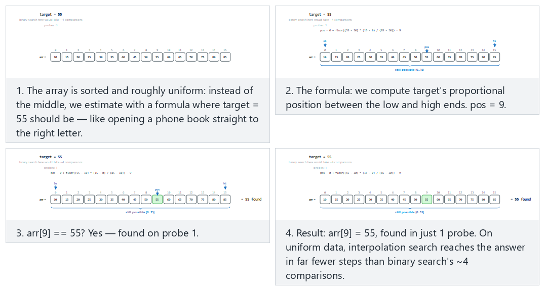
In the picker, also try slightly uneven spacing, needs a few probes (hard) and the edge cases skewed data: last value is huge, many probes, all values equal: the division guard kicks in, and target is entirely outside the range: rejected on sight — or press 🎲 for random data, or type your own sorted array.
3.5 Try it
Full program: interpolation_search.c / InterpolationSearch.java
/* Week 6 -- Search and Hashing
 * Interpolation search: on a SORTED, roughly uniform array, estimate where
 * the target should be with a formula instead of always checking the
 * middle. A guard avoids dividing by zero when the current range is all one
 * value. Prints every probe.
 * CEN207 Data Structures (formerly CE205)
 */
#include <stdio.h>

int interpolation_search(const int arr[], int n, int target, int *probes) {
    int lo = 0, hi = n - 1, p = 0;
    while (lo <= hi && target >= arr[lo] && target <= arr[hi]) {
        p++;
        if (arr[hi] == arr[lo]) {                 /* guard: avoid division by zero */
            printf("  probe %d: arr[hi] == arr[lo] (%d), guard triggered\n", p, arr[lo]);
            *probes = p;
            return lo;                            /* target must equal arr[lo] here */
        }
        /* widen to long long: target-arr[lo] and arr[hi]-arr[lo] can overflow a 32-bit int
           when the array spans values near INT_MIN and INT_MAX at once */
        long long span = (long long) arr[hi] - (long long) arr[lo];
        long long num = (long long) target - (long long) arr[lo];
        int pos = lo + (int) ((double) num * (hi - lo) / (double) span);
        printf("  probe %d: lo=%d hi=%d pos=%d arr[pos]=%d\n", p, lo, hi, pos, arr[pos]);
        if (arr[pos] == target) { *probes = p; return pos; }
        if (arr[pos] < target) lo = pos + 1;
        else hi = pos - 1;
    }
    *probes = p;
    return -1;
}

static void print_array(const int arr[], int n) {
    printf("arr =");
    for (int i = 0; i < n; i++) printf(" %d", arr[i]);
    printf("\n");
}

static void run_scenario(const char *label, const int arr[], int n, int target) {
    printf("-- %s --\n", label);
    print_array(arr, n);
    printf("target = %d\n", target);
    int probes = 0;
    int index = interpolation_search(arr, n, target, &probes);
    if (index == -1) printf("result: not found, %d probes\n\n", probes);
    else printf("result: found at index %d, %d probes\n\n", index, probes);
}

int main(void) {
    int normal[] = {10, 15, 20, 25, 30, 35, 40, 45, 50, 55, 60, 65, 70, 75, 80, 85};
    int hard[] = {10, 13, 21, 24, 33, 36, 44, 48, 55, 61, 68, 74, 81, 87, 94, 100};
    int skewed[] = {1, 2, 3, 4, 5, 6, 7, 8, 9, 10, 11, 12, 13, 14, 15, 1000000};
    int all_equal[] = {42, 42, 42, 42, 42, 42, 42, 42, 42, 42, 42, 42, 42, 42, 42, 42};

    run_scenario("normal: uniformly spread 16 values, found in a single probe", normal, 16, 55);
    run_scenario("hard: slightly uneven spacing, needs a few probes", hard, 16, 81);
    run_scenario("edge: skewed data, last value is huge, many probes", skewed, 16, 8);
    run_scenario("edge: all values equal, the division guard kicks in", all_equal, 16, 42);
    run_scenario("edge: target is entirely outside the range, rejected on sight", normal, 16, 999);

    return 0;
}
/* Week 6 -- Search and Hashing
 * Interpolation search: on a SORTED, roughly uniform array, estimate where
 * the target should be with a formula instead of always checking the
 * middle. A guard avoids dividing by zero when the current range is all one
 * value. Prints every probe.
 * CEN207 Data Structures (formerly CE205)
 */
public class InterpolationSearch {
    static int probes;

    static int interpolationSearch(int[] arr, int target) {
        int lo = 0, hi = arr.length - 1;
        probes = 0;
        while (lo <= hi && target >= arr[lo] && target <= arr[hi]) {
            probes++;
            if (arr[hi] == arr[lo]) {                 // guard: avoid division by zero
                System.out.println("  probe " + probes + ": arr[hi] == arr[lo] (" + arr[lo] + "), guard triggered");
                return lo;                            // target must equal arr[lo] here
            }
            // widen to long: target-arr[lo] and arr[hi]-arr[lo] can overflow a 32-bit int
            // when the array spans values near Integer.MIN_VALUE and Integer.MAX_VALUE at once
            long span = (long) arr[hi] - (long) arr[lo];
            long num = (long) target - (long) arr[lo];
            int pos = lo + (int) ((double) num * (hi - lo) / (double) span);
            System.out.println("  probe " + probes + ": lo=" + lo + " hi=" + hi + " pos=" + pos + " arr[pos]=" + arr[pos]);
            if (arr[pos] == target) return pos;
            if (arr[pos] < target) lo = pos + 1;
            else hi = pos - 1;
        }
        return -1;
    }

    static void printArray(int[] arr) {
        StringBuilder sb = new StringBuilder("arr =");
        for (int v : arr) sb.append(' ').append(v);
        System.out.println(sb);
    }

    static void runScenario(String label, int[] arr, int target) {
        System.out.println("-- " + label + " --");
        printArray(arr);
        System.out.println("target = " + target);
        int index = interpolationSearch(arr, target);
        if (index == -1) System.out.println("result: not found, " + probes + " probes");
        else System.out.println("result: found at index " + index + ", " + probes + " probes");
        System.out.println();
    }

    public static void main(String[] args) {
        int[] normal = {10, 15, 20, 25, 30, 35, 40, 45, 50, 55, 60, 65, 70, 75, 80, 85};
        int[] hard = {10, 13, 21, 24, 33, 36, 44, 48, 55, 61, 68, 74, 81, 87, 94, 100};
        int[] skewed = {1, 2, 3, 4, 5, 6, 7, 8, 9, 10, 11, 12, 13, 14, 15, 1000000};
        int[] allEqual = {42, 42, 42, 42, 42, 42, 42, 42, 42, 42, 42, 42, 42, 42, 42, 42};

        runScenario("normal: uniformly spread 16 values, found in a single probe", normal, 55);
        runScenario("hard: slightly uneven spacing, needs a few probes", hard, 81);
        runScenario("edge: skewed data, last value is huge, many probes", skewed, 8);
        runScenario("edge: all values equal, the division guard kicks in", allEqual, 42);
        runScenario("edge: target is entirely outside the range, rejected on sight", normal, 999);
    }
}
Try it
Expected output:
-- normal: uniformly spread 16 values, found in a single probe --
arr = 10 15 20 25 30 35 40 45 50 55 60 65 70 75 80 85
target = 55
  probe 1: lo=0 hi=15 pos=9 arr[pos]=55
result: found at index 9, 1 probes

-- hard: slightly uneven spacing, needs a few probes --
arr = 10 13 21 24 33 36 44 48 55 61 68 74 81 87 94 100
target = 81
  probe 1: lo=0 hi=15 pos=11 arr[pos]=74
  probe 2: lo=12 hi=15 pos=12 arr[pos]=81
result: found at index 12, 2 probes

-- edge: skewed data, last value is huge, many probes --
arr = 1 2 3 4 5 6 7 8 9 10 11 12 13 14 15 1000000
target = 8
  probe 1: lo=0 hi=15 pos=0 arr[pos]=1
  probe 2: lo=1 hi=15 pos=1 arr[pos]=2
  probe 3: lo=2 hi=15 pos=2 arr[pos]=3
  probe 4: lo=3 hi=15 pos=3 arr[pos]=4
  probe 5: lo=4 hi=15 pos=4 arr[pos]=5
  probe 6: lo=5 hi=15 pos=5 arr[pos]=6
  probe 7: lo=6 hi=15 pos=6 arr[pos]=7
  probe 8: lo=7 hi=15 pos=7 arr[pos]=8
result: found at index 7, 8 probes

-- edge: all values equal, the division guard kicks in --
arr = 42 42 42 42 42 42 42 42 42 42 42 42 42 42 42 42
target = 42
  probe 1: arr[hi] == arr[lo] (42), guard triggered
result: found at index 0, 1 probes

-- edge: target is entirely outside the range, rejected on sight --
arr = 10 15 20 25 30 35 40 45 50 55 60 65 70 75 80 85
target = 999
result: not found, 0 probes
3.6 Complexity, mistakes, self-check
Complexity. Average case O(log log n) on uniformly distributed data; worst case O(n) on skewed data (the array [1, 2, 3, ..., 15, 1000000] above needed 8 probes for just 16 elements — imagine the same shape scaled up to a million elements). Needs a sorted array, exactly like binary search.
Common mistakes
- Forgetting the
arr[hi] == arr[lo]guard. Without it, a range of repeated values causes a division by zero. This is not a rare edge case in practice — any real dataset with duplicate values can trigger it once the search narrows down far enough. - Using integer division without casting to
doublefirst.(target - arr[lo]) * (hi - lo) / (arr[hi] - arr[lo])computed entirely inintarithmetic can overflow for large key ranges, and loses the fractional precision the formula depends on; casting the numerator todouble(as the code above does) avoids both problems. - Assuming interpolation search is always faster than binary search. It is a bet that pays off only on roughly uniform data; on skewed or adversarial data it can be dramatically slower. Never use it blindly on data whose distribution you have not checked.
Self-check: why the guard returns lo, not "not found"
In the "all values equal" scenario above, the guard triggers immediately and returns index 0 (lo) as a found result. Why is that correct, given that the guard fires the instant arr[hi] == arr[lo], before ever comparing arr[lo] to target?
Answer. The while loop's own condition already guarantees target >= arr[lo] && target <= arr[hi] before the guard is even reached. If, in addition, arr[hi] == arr[lo], then arr[lo] and arr[hi] are the same value, and target is sandwiched between two equal bounds — so target must equal that value too. Returning lo is therefore always correct in this branch, without needing a separate comparison.
4. Exponential search
4.1 A question to start
Binary search needs to know n, the array's size, before it starts, to compute the first midpoint. But what if the array is effectively unbounded — a sorted stream, or an array so enormous that just reading n is itself expensive — and you strongly suspect the target, if present, is somewhere near the front? Scanning the whole thing to find n first would be wasteful. Exponential search solves this: find a bound that is guaranteed to contain the target by doubling (1, 2, 4, 8, …) until you overshoot it, then run ordinary binary search inside that bound. The bound-finding phase costs only O(log index) — proportional to how far in the target actually is — not O(log n).
Jon Bentley and Andrew Yao published this technique in their 1976 paper An Almost Optimal Algorithm for Unbounded Searching (Information Processing Letters). It is also called unbounded search or galloping search — "galloping" for the doubling bound-finding phase, small steps that grow larger and larger like a horse picking up speed — and variants of it are used today inside several merge and set-intersection algorithms.
4.2 The idea: double until you overshoot, then binary search
Check arr[0] first (comparison #1). If it is not the target, grow a bound by doubling — 1, 2, 4, 8, … — checking arr[bound] each time, until arr[bound] >= target or bound >= n. At that point, target, if present, must lie in [bound/2, min(bound, n-1)] — because the previous, smaller bound was checked and found < target. Run ordinary binary search inside exactly that range.
4.3 In memory, and the code
int exponential_search(const int arr[], int n, int target, int *comparisons) {
    if (n <= 0) { *comparisons = 0; return -1; }    /* nothing to search */
    int comp = 1;                    /* the arr[0] check below counts as comparison #1 */
    if (arr[0] == target) { *comparisons = comp; return 0; }
    int bound = 1;
    while (bound < n) {                 /* double the bound until it overshoots target */
        comp++;
        if (arr[bound] >= target) break;
        bound *= 2;
    }
    int lo = bound / 2, hi = (bound < n) ? bound : n - 1;
    while (lo <= hi) {                  /* ordinary binary search inside [lo..hi] */
        int mid = lo + (hi - lo) / 2;
        comp++;
        if (arr[mid] == target) { *comparisons = comp; return mid; }
        if (arr[mid] < target) lo = mid + 1;
        else hi = mid - 1;
    }
    *comparisons = comp;
    return -1;
}
static int exponentialSearch(int[] arr, int target) {
    int n = arr.length;
    if (n <= 0) { comparisons = 0; return -1; }  // nothing to search
    comparisons = 1;                 // the arr[0] check below counts as comparison #1
    if (arr[0] == target) return 0;
    int bound = 1;
    while (bound < n) {                 // double the bound until it overshoots target
        comparisons++;
        if (arr[bound] >= target) break;
        bound *= 2;
    }
    int lo = bound / 2, hi = (bound < n) ? bound : n - 1;
    while (lo <= hi) {                  // ordinary binary search inside [lo..hi]
        int mid = lo + (hi - lo) / 2;
        comparisons++;
        if (arr[mid] == target) return mid;
        if (arr[mid] < target) lo = mid + 1;
        else hi = mid - 1;
    }
    return -1;
}
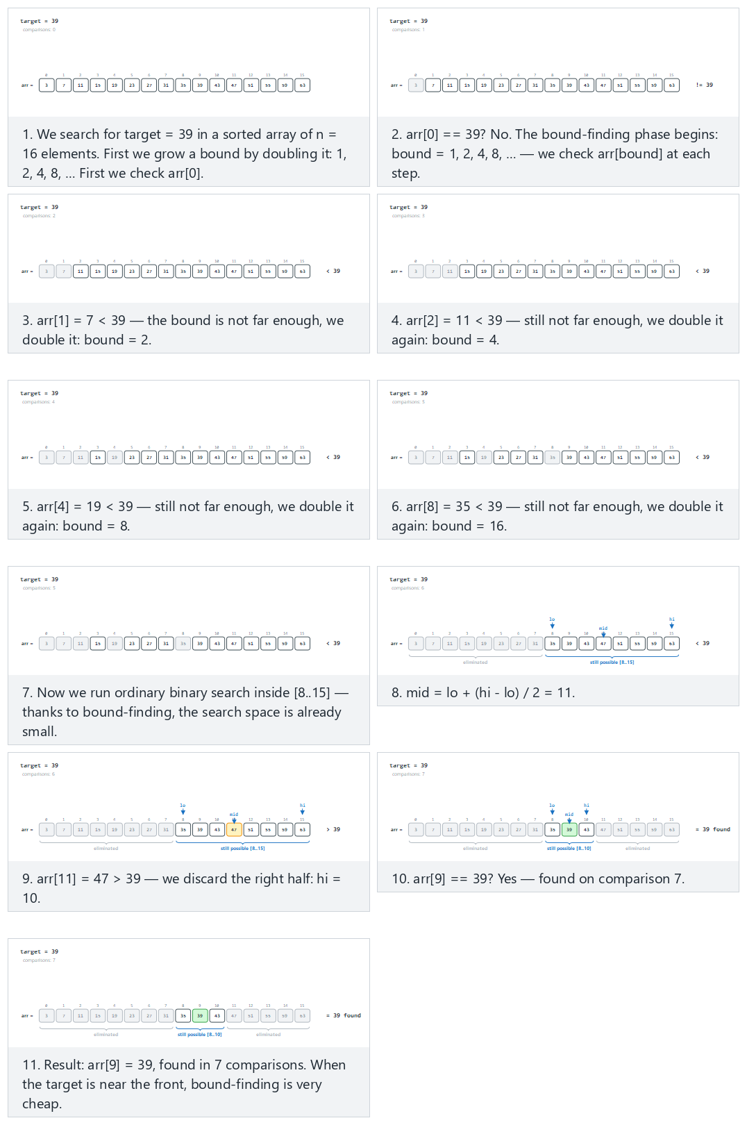
In the picker, also try target near the end, the bound doubles several times (hard) and the edge cases target is the first element: a single comparison, target is larger than the last element, and target is in range but not in the array — or press 🎲 for random data, or type your own sorted array.
4.4 Try it
Full program: exponential_search.c / ExponentialSearch.java
/* Week 6 -- Search and Hashing
 * Exponential search: on a SORTED array, double a bound (1, 2, 4, 8, ...)
 * until it overshoots target, then run ordinary binary search inside
 * [bound/2, bound]. Prints the bound-finding phase and the binary-search
 * phase.
 * CEN207 Data Structures (formerly CE205)
 */
#include <stdio.h>

int exponential_search(const int arr[], int n, int target, int *comparisons) {
    if (n <= 0) { *comparisons = 0; return -1; }    /* nothing to search */
    int comp = 1;                    /* the arr[0] check below counts as comparison #1 */
    printf("  check arr[0] = %d\n", arr[0]);
    if (arr[0] == target) { *comparisons = comp; return 0; }
    int bound = 1;
    while (bound < n) {                 /* double the bound until it overshoots target */
        comp++;
        printf("  bound = %d: check arr[%d] = %d\n", bound, bound, arr[bound]);
        if (arr[bound] >= target) break;
        bound *= 2;
    }
    int lo = bound / 2, hi = (bound < n) ? bound : n - 1;
    printf("  binary search inside [%d..%d]\n", lo, hi);
    while (lo <= hi) {                  /* ordinary binary search inside [lo..hi] */
        int mid = lo + (hi - lo) / 2;
        comp++;
        printf("  compare arr[%d] = %d\n", mid, arr[mid]);
        if (arr[mid] == target) { *comparisons = comp; return mid; }
        if (arr[mid] < target) lo = mid + 1;
        else hi = mid - 1;
    }
    *comparisons = comp;
    return -1;
}

static void print_array(const int arr[], int n) {
    printf("arr =");
    for (int i = 0; i < n; i++) printf(" %d", arr[i]);
    printf("\n");
}

static void run_scenario(const char *label, const int arr[], int n, int target) {
    printf("-- %s --\n", label);
    print_array(arr, n);
    printf("target = %d\n", target);
    int comparisons = 0;
    int index = exponential_search(arr, n, target, &comparisons);
    if (index == -1) printf("result: not found, %d comparisons\n\n", comparisons);
    else printf("result: found at index %d, %d comparisons\n\n", index, comparisons);
}

int main(void) {
    int a[] = {3, 7, 11, 15, 19, 23, 27, 31, 35, 39, 43, 47, 51, 55, 59, 63};
    int n = 16;

    run_scenario("normal: 16 values, target found around the middle", a, n, 39);
    run_scenario("hard: target near the end, the bound doubles several times", a, n, 59);
    run_scenario("edge: target is the first element, a single comparison", a, n, 3);
    run_scenario("edge: target is larger than the last element", a, n, 999);
    run_scenario("edge: target is in range but not in the array", a, n, 40);

    return 0;
}
/* Week 6 -- Search and Hashing
 * Exponential search: on a SORTED array, double a bound (1, 2, 4, 8, ...)
 * until it overshoots target, then run ordinary binary search inside
 * [bound/2, bound]. Prints the bound-finding phase and the binary-search
 * phase.
 * CEN207 Data Structures (formerly CE205)
 */
public class ExponentialSearch {
    static int comparisons;

    static int exponentialSearch(int[] arr, int target) {
        int n = arr.length;
        if (n <= 0) { comparisons = 0; return -1; }  // nothing to search
        comparisons = 1;                 // the arr[0] check below counts as comparison #1
        System.out.println("  check arr[0] = " + arr[0]);
        if (arr[0] == target) return 0;
        int bound = 1;
        while (bound < n) {                 // double the bound until it overshoots target
            comparisons++;
            System.out.println("  bound = " + bound + ": check arr[" + bound + "] = " + arr[bound]);
            if (arr[bound] >= target) break;
            bound *= 2;
        }
        int lo = bound / 2, hi = (bound < n) ? bound : n - 1;
        System.out.println("  binary search inside [" + lo + ".." + hi + "]");
        while (lo <= hi) {                  // ordinary binary search inside [lo..hi]
            int mid = lo + (hi - lo) / 2;
            comparisons++;
            System.out.println("  compare arr[" + mid + "] = " + arr[mid]);
            if (arr[mid] == target) return mid;
            if (arr[mid] < target) lo = mid + 1;
            else hi = mid - 1;
        }
        return -1;
    }

    static void printArray(int[] arr) {
        StringBuilder sb = new StringBuilder("arr =");
        for (int v : arr) sb.append(' ').append(v);
        System.out.println(sb);
    }

    static void runScenario(String label, int[] arr, int target) {
        System.out.println("-- " + label + " --");
        printArray(arr);
        System.out.println("target = " + target);
        int index = exponentialSearch(arr, target);
        if (index == -1) System.out.println("result: not found, " + comparisons + " comparisons");
        else System.out.println("result: found at index " + index + ", " + comparisons + " comparisons");
        System.out.println();
    }

    public static void main(String[] args) {
        int[] a = {3, 7, 11, 15, 19, 23, 27, 31, 35, 39, 43, 47, 51, 55, 59, 63};

        runScenario("normal: 16 values, target found around the middle", a, 39);
        runScenario("hard: target near the end, the bound doubles several times", a, 59);
        runScenario("edge: target is the first element, a single comparison", a, 3);
        runScenario("edge: target is larger than the last element", a, 999);
        runScenario("edge: target is in range but not in the array", a, 40);
    }
}
Try it
Expected output:
-- normal: 16 values, target found around the middle --
arr = 3 7 11 15 19 23 27 31 35 39 43 47 51 55 59 63
target = 39
  check arr[0] = 3
  bound = 1: check arr[1] = 7
  bound = 2: check arr[2] = 11
  bound = 4: check arr[4] = 19
  bound = 8: check arr[8] = 35
  binary search inside [8..15]
  compare arr[11] = 47
  compare arr[9] = 39
result: found at index 9, 7 comparisons

-- hard: target near the end, the bound doubles several times --
arr = 3 7 11 15 19 23 27 31 35 39 43 47 51 55 59 63
target = 59
  check arr[0] = 3
  bound = 1: check arr[1] = 7
  bound = 2: check arr[2] = 11
  bound = 4: check arr[4] = 19
  bound = 8: check arr[8] = 35
  binary search inside [8..15]
  compare arr[11] = 47
  compare arr[13] = 55
  compare arr[14] = 59
result: found at index 14, 8 comparisons

-- edge: target is the first element, a single comparison --
arr = 3 7 11 15 19 23 27 31 35 39 43 47 51 55 59 63
target = 3
  check arr[0] = 3
result: found at index 0, 1 comparisons

-- edge: target is larger than the last element --
arr = 3 7 11 15 19 23 27 31 35 39 43 47 51 55 59 63
target = 999
  check arr[0] = 3
  bound = 1: check arr[1] = 7
  bound = 2: check arr[2] = 11
  bound = 4: check arr[4] = 19
  bound = 8: check arr[8] = 35
  binary search inside [8..15]
  compare arr[11] = 47
  compare arr[13] = 55
  compare arr[14] = 59
  compare arr[15] = 63
result: not found, 9 comparisons

-- edge: target is in range but not in the array --
arr = 3 7 11 15 19 23 27 31 35 39 43 47 51 55 59 63
target = 40
  check arr[0] = 3
  bound = 1: check arr[1] = 7
  bound = 2: check arr[2] = 11
  bound = 4: check arr[4] = 19
  bound = 8: check arr[8] = 35
  binary search inside [8..15]
  compare arr[11] = 47
  compare arr[9] = 39
  compare arr[10] = 43
result: not found, 8 comparisons
4.5 Complexity, mistakes, self-check
Complexity. O(log index) to find the bound, where index is the target's actual position (or n if absent) — not O(log n). The binary-search phase then costs O(log(bound)), where bound is at most 2 * index. Combined: O(log index) overall. When the target is near the front, this beats plain binary search's O(log n); when the target is near the end, the two become asymptotically the same.
Common mistakes
- Forgetting to clamp
hiton - 1after the bound-finding loop.boundcan legitimately exceedn - 1(the loop's own condition isbound < n, but the last doubling can still pushboundpast the array), so the binary search'shimust bemin(bound, n - 1), notbounditself, or it reads out of bounds. - Starting the doubling loop at
bound = 0instead ofbound = 1. Doubling0stays0forever — an infinite loop.arr[0]is already handled separately before the loop starts, so the loop must begin atbound = 1. - Re-deriving
loincorrectly. The correct lower bound for the binary-search phase isbound / 2(the previous bound, which was already checked and confirmed< target), not0and notbounditself — using the wronglothrows away the very savings exponential search exists to provide.
Self-check: exponential search versus binary search
For an array of a million elements, roughly how many comparisons does exponential search need if the target is at index 5 (near the very front), versus if the target is at index 999,999 (the very last element)? Compare both to plain binary search's roughly 20 comparisons.
Answer. Near the front (index 5): the bound-finding phase only needs to double past 5 — 1, 2, 4, 8 — about 4 comparisons, then binary search inside [4..8] costs about log2(5) ≈ 3 more: roughly 7 comparisons total, far fewer than binary search's 20. Near the very end (index 999,999): the bound-finding phase must double all the way past a million — 1, 2, 4, ..., 2^20 — about 20 comparisons, then binary search inside a range of comparable size costs about 20 more: roughly 40 comparisons total, worse than plain binary search's 20. Exponential search is a specialized tool for "probably near the front", not a universal replacement for binary search.
5. Fibonacci search
5.1 A question to start
Binary search's midpoint computation, lo + (hi - lo) / 2, needs a division. On computing hardware from the 1950s and 1960s — and still today on some very constrained embedded processors — division is dramatically more expensive than addition or subtraction. Is there a way to get binary search's O(log n) guarantee using only addition and subtraction? Fibonacci search answers yes, by splitting the search range according to Fibonacci numbers (1, 1, 2, 3, 5, 8, 13, 21, …) instead of always splitting it exactly in half.
The technique traces back to work by the American statistician Jack Kiefer, whose 1953 paper Sequential Minimax Search for a Maximum used Fibonacci numbers to design an optimal strategy for a related problem (finding the maximum of a function using as few evaluations as possible); the same Fibonacci-number splitting idea was later adapted into a division-free search algorithm for sorted arrays, which is what you are learning here.
5.2 The idea
Find the smallest Fibonacci number fib that is >= n, together with the two Fibonacci numbers just before it, fib1 and fib2 (so fib = fib1 + fib2). Maintain an offset (initially -1) marking how far into the array the search has already eliminated. At each step, probe index i = offset + fib2 (clamped to n - 1 if that would overshoot). If arr[i] < target, the entire left part up to i is eliminated, offset moves to i, and the Fibonacci triple shrinks by one step (fib, fib1, fib2 = fib1, fib2, fib1 - fib2). If arr[i] > target, the right part is eliminated instead, and the triple shrinks by two steps (fib, fib1, fib2 = fib2, fib1 - fib2, fib - (fib1 - fib2)). Because Fibonacci numbers satisfy fib = fib1 + fib2 exactly, every one of these updates uses only addition and subtraction — never a division or a multiplication.
5.3 In memory, and the code
int fibonacci_search(const int arr[], int n, int target, int *comparisons) {
    int fib2 = 0, fib1 = 1, fib = fib1 + fib2;      /* smallest Fibonacci number >= n */
    while (fib < n) { fib2 = fib1; fib1 = fib; fib = fib1 + fib2; }
    int offset = -1, comp = 0;
    while (fib > 1) {
        int i = (offset + fib2 < n - 1) ? offset + fib2 : n - 1;
        comp++;
        if (arr[i] < target) {                       /* eliminate the left part */
            fib = fib1; fib1 = fib2; fib2 = fib - fib1;
            offset = i;
        } else if (arr[i] > target) {                /* eliminate the right part */
            fib = fib2; fib1 = fib1 - fib2; fib2 = fib - fib1;
        } else {
            *comparisons = comp;
            return i;
        }
    }
    if (fib1 == 1 && offset + 1 < n) {                /* one element may be left over */
        comp++;
        if (arr[offset + 1] == target) { *comparisons = comp; return offset + 1; }
    }
    *comparisons = comp;
    return -1;
}
static int fibonacciSearch(int[] arr, int target) {
    int n = arr.length;
    int fib2 = 0, fib1 = 1, fib = fib1 + fib2;      // smallest Fibonacci number >= n
    while (fib < n) { fib2 = fib1; fib1 = fib; fib = fib1 + fib2; }
    int offset = -1;
    comparisons = 0;
    while (fib > 1) {
        int i = (offset + fib2 < n - 1) ? offset + fib2 : n - 1;
        comparisons++;
        if (arr[i] < target) {                       // eliminate the left part
            fib = fib1; fib1 = fib2; fib2 = fib - fib1;
            offset = i;
        } else if (arr[i] > target) {                // eliminate the right part
            fib = fib2; fib1 = fib1 - fib2; fib2 = fib - fib1;
        } else {
            return i;
        }
    }
    if (fib1 == 1 && offset + 1 < n) {                // one element may be left over
        comparisons++;
        if (arr[offset + 1] == target) return offset + 1;
    }
    return -1;
}
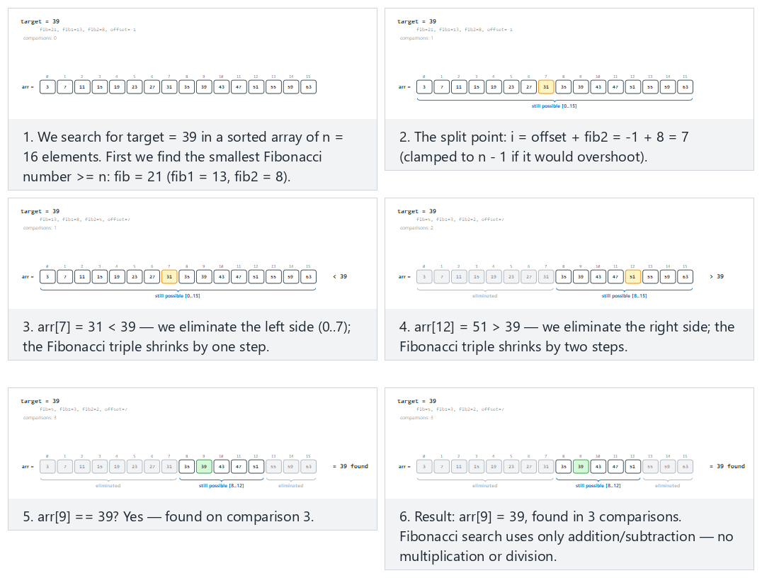
In the picker, also try target near the end, needs several splits (hard) and the edge cases target is the first element, target is larger than the last element, and target is in range but not in the array — or press 🎲 for random data, or type your own sorted array.
5.4 Try it
Full program: fibonacci_search.c / FibonacciSearch.java
/* Week 6 -- Search and Hashing
 * Fibonacci search: on a SORTED array, split the range using Fibonacci
 * numbers instead of the middle (binary search) or a formula
 * (interpolation search). Uses only addition and subtraction. Prints the
 * Fibonacci triple and every probe.
 * CEN207 Data Structures (formerly CE205)
 */
#include <stdio.h>

int fibonacci_search(const int arr[], int n, int target, int *comparisons) {
    int fib2 = 0, fib1 = 1, fib = fib1 + fib2;      /* smallest Fibonacci number >= n */
    while (fib < n) { int t = fib1 + fib; fib2 = fib1; fib1 = fib; fib = t; }
    printf("  smallest fib >= n: fib=%d fib1=%d fib2=%d\n", fib, fib1, fib2);

    int offset = -1, comp = 0;
    while (fib > 1) {
        int i = (offset + fib2 < n - 1) ? offset + fib2 : n - 1;
        comp++;
        printf("  probe %d: i=%d arr[i]=%d (fib=%d fib1=%d fib2=%d offset=%d)\n",
               comp, i, arr[i], fib, fib1, fib2, offset);
        if (arr[i] < target) {                       /* eliminate the left part */
            fib = fib1; fib1 = fib2; fib2 = fib - fib1;
            offset = i;
        } else if (arr[i] > target) {                /* eliminate the right part */
            fib = fib2; fib1 = fib1 - fib2; fib2 = fib - fib1;
        } else {
            *comparisons = comp;
            return i;
        }
    }
    if (fib1 == 1 && offset + 1 < n) {                /* one element may be left over */
        comp++;
        printf("  probe %d: one element left over, i=%d arr[i]=%d\n", comp, offset + 1, arr[offset + 1]);
        if (arr[offset + 1] == target) { *comparisons = comp; return offset + 1; }
    }
    *comparisons = comp;
    return -1;
}

static void print_array(const int arr[], int n) {
    printf("arr =");
    for (int i = 0; i < n; i++) printf(" %d", arr[i]);
    printf("\n");
}

static void run_scenario(const char *label, const int arr[], int n, int target) {
    printf("-- %s --\n", label);
    print_array(arr, n);
    printf("target = %d\n", target);
    int comparisons = 0;
    int index = fibonacci_search(arr, n, target, &comparisons);
    if (index == -1) printf("result: not found, %d comparisons\n\n", comparisons);
    else printf("result: found at index %d, %d comparisons\n\n", index, comparisons);
}

int main(void) {
    int a[] = {3, 7, 11, 15, 19, 23, 27, 31, 35, 39, 43, 47, 51, 55, 59, 63};
    int n = 16;

    run_scenario("normal: 16 values, target found around the middle", a, n, 39);
    run_scenario("hard: target near the end, needs several splits", a, n, 59);
    run_scenario("edge: target is the first element", a, n, 3);
    run_scenario("edge: target is larger than the last element", a, n, 999);
    run_scenario("edge: target is in range but not in the array", a, n, 40);

    return 0;
}
/* Week 6 -- Search and Hashing
 * Fibonacci search: on a SORTED array, split the range using Fibonacci
 * numbers instead of the middle (binary search) or a formula
 * (interpolation search). Uses only addition and subtraction. Prints the
 * Fibonacci triple and every probe.
 * CEN207 Data Structures (formerly CE205)
 */
public class FibonacciSearch {
    static int comparisons;

    static int fibonacciSearch(int[] arr, int target) {
        int n = arr.length;
        int fib2 = 0, fib1 = 1, fib = fib1 + fib2;      // smallest Fibonacci number >= n
        while (fib < n) { int t = fib1 + fib; fib2 = fib1; fib1 = fib; fib = t; }
        System.out.println("  smallest fib >= n: fib=" + fib + " fib1=" + fib1 + " fib2=" + fib2);

        int offset = -1;
        comparisons = 0;
        while (fib > 1) {
            int i = (offset + fib2 < n - 1) ? offset + fib2 : n - 1;
            comparisons++;
            System.out.println("  probe " + comparisons + ": i=" + i + " arr[i]=" + arr[i]
                    + " (fib=" + fib + " fib1=" + fib1 + " fib2=" + fib2 + " offset=" + offset + ")");
            if (arr[i] < target) {                       // eliminate the left part
                fib = fib1; fib1 = fib2; fib2 = fib - fib1;
                offset = i;
            } else if (arr[i] > target) {                // eliminate the right part
                fib = fib2; fib1 = fib1 - fib2; fib2 = fib - fib1;
            } else {
                return i;
            }
        }
        if (fib1 == 1 && offset + 1 < n) {                // one element may be left over
            comparisons++;
            System.out.println("  probe " + comparisons + ": one element left over, i=" + (offset + 1) + " arr[i]=" + arr[offset + 1]);
            if (arr[offset + 1] == target) return offset + 1;
        }
        return -1;
    }

    static void printArray(int[] arr) {
        StringBuilder sb = new StringBuilder("arr =");
        for (int v : arr) sb.append(' ').append(v);
        System.out.println(sb);
    }

    static void runScenario(String label, int[] arr, int target) {
        System.out.println("-- " + label + " --");
        printArray(arr);
        System.out.println("target = " + target);
        int index = fibonacciSearch(arr, target);
        if (index == -1) System.out.println("result: not found, " + comparisons + " comparisons");
        else System.out.println("result: found at index " + index + ", " + comparisons + " comparisons");
        System.out.println();
    }

    public static void main(String[] args) {
        int[] a = {3, 7, 11, 15, 19, 23, 27, 31, 35, 39, 43, 47, 51, 55, 59, 63};

        runScenario("normal: 16 values, target found around the middle", a, 39);
        runScenario("hard: target near the end, needs several splits", a, 59);
        runScenario("edge: target is the first element", a, 3);
        runScenario("edge: target is larger than the last element", a, 999);
        runScenario("edge: target is in range but not in the array", a, 40);
    }
}
Try it
Expected output:
-- normal: 16 values, target found around the middle --
arr = 3 7 11 15 19 23 27 31 35 39 43 47 51 55 59 63
target = 39
  smallest fib >= n: fib=21 fib1=13 fib2=8
  probe 1: i=7 arr[i]=31 (fib=21 fib1=13 fib2=8 offset=-1)
  probe 2: i=12 arr[i]=51 (fib=13 fib1=8 fib2=5 offset=7)
  probe 3: i=9 arr[i]=39 (fib=5 fib1=3 fib2=2 offset=7)
result: found at index 9, 3 comparisons

-- hard: target near the end, needs several splits --
arr = 3 7 11 15 19 23 27 31 35 39 43 47 51 55 59 63
target = 59
  smallest fib >= n: fib=21 fib1=13 fib2=8
  probe 1: i=7 arr[i]=31 (fib=21 fib1=13 fib2=8 offset=-1)
  probe 2: i=12 arr[i]=51 (fib=13 fib1=8 fib2=5 offset=7)
  probe 3: i=15 arr[i]=63 (fib=8 fib1=5 fib2=3 offset=12)
  probe 4: i=13 arr[i]=55 (fib=3 fib1=2 fib2=1 offset=12)
  probe 5: i=14 arr[i]=59 (fib=2 fib1=1 fib2=1 offset=13)
result: found at index 14, 5 comparisons

-- edge: target is the first element --
arr = 3 7 11 15 19 23 27 31 35 39 43 47 51 55 59 63
target = 3
  smallest fib >= n: fib=21 fib1=13 fib2=8
  probe 1: i=7 arr[i]=31 (fib=21 fib1=13 fib2=8 offset=-1)
  probe 2: i=2 arr[i]=11 (fib=8 fib1=5 fib2=3 offset=-1)
  probe 3: i=0 arr[i]=3 (fib=3 fib1=2 fib2=1 offset=-1)
result: found at index 0, 3 comparisons

-- edge: target is larger than the last element --
arr = 3 7 11 15 19 23 27 31 35 39 43 47 51 55 59 63
target = 999
  smallest fib >= n: fib=21 fib1=13 fib2=8
  probe 1: i=7 arr[i]=31 (fib=21 fib1=13 fib2=8 offset=-1)
  probe 2: i=12 arr[i]=51 (fib=13 fib1=8 fib2=5 offset=7)
  probe 3: i=15 arr[i]=63 (fib=8 fib1=5 fib2=3 offset=12)
  probe 4: i=15 arr[i]=63 (fib=5 fib1=3 fib2=2 offset=15)
  probe 5: i=15 arr[i]=63 (fib=3 fib1=2 fib2=1 offset=15)
  probe 6: i=15 arr[i]=63 (fib=2 fib1=1 fib2=1 offset=15)
result: not found, 6 comparisons

-- edge: target is in range but not in the array --
arr = 3 7 11 15 19 23 27 31 35 39 43 47 51 55 59 63
target = 40
  smallest fib >= n: fib=21 fib1=13 fib2=8
  probe 1: i=7 arr[i]=31 (fib=21 fib1=13 fib2=8 offset=-1)
  probe 2: i=12 arr[i]=51 (fib=13 fib1=8 fib2=5 offset=7)
  probe 3: i=9 arr[i]=39 (fib=5 fib1=3 fib2=2 offset=7)
  probe 4: i=10 arr[i]=43 (fib=3 fib1=2 fib2=1 offset=9)
  probe 5: one element left over, i=10 arr[i]=43
result: not found, 5 comparisons
5.5 Complexity, mistakes, self-check
Complexity. O(log n) worst case, same asymptotic class as binary search, since consecutive Fibonacci numbers grow at the same exponential rate as powers of two (the ratio fib(k+1) / fib(k) converges to the golden ratio, about 1.618, a constant just like binary search's 2). The entire algorithm uses only addition and subtraction — never multiplication or division — which was Fibonacci search's original selling point on hardware where division was slow or unavailable.
Common mistakes
- Confusing which side eliminates one step versus two. Eliminating the left part shrinks the Fibonacci triple by one step (
fib, fib1, fib2 -> fib1, fib2, fib - fib1); eliminating the right part shrinks it by two steps (fib, fib1, fib2 -> fib2, fib1 - fib2, ...). Swapping these breaks the algorithm's correctness, not just its performance. - Forgetting the leftover-element check after the main loop. Because
fibshrinks in whole Fibonacci steps rather than exactly halving, the loop can end withfib1 == 1and one array position never yet compared — the finalifblock above catches exactly that case. - Recomputing the Fibonacci sequence from scratch on every probe. The whole point of maintaining
fib,fib1,fib2incrementally is to avoid ever calling a Fibonacci-computing function inside the loop; recomputing it every time turns an O(1)-per-step update into unnecessary extra work.
Self-check: why does this need no division?
Binary search's midpoint is lo + (hi - lo) / 2 — a division by 2. Fibonacci search's probe index is offset + fib2. Where did the "divide the range in some proportion" step go, and why does maintaining fib, fib1, fib2 incrementally avoid ever needing it?
Answer. Because fib = fib1 + fib2 always holds, fib2 already represents (approximately) the Fibonacci-ratio-sized fraction of the current range — no division needed to compute it, because it was never computed by dividing fib in the first place; it is tracked directly as one of the three running numbers, updated by pure addition and subtraction at every step. The "division" work that binary search does at every probe is instead done once, up front, when finding the smallest Fibonacci number >= n (a loop of additions), and never again.
6. Comparison table of search methods
| Method | Requires sorted? | Worst case | Best/typical case | Extra assumption | Arithmetic per step |
|---|---|---|---|---|---|
| Linear search (Week 1) | No | O(n) | O(n) | None | Comparison only |
| Binary search (Week 1) | Yes | O(log n) | O(log n) | None | One division/shift |
| Jump search | Yes | O(sqrt n) | O(sqrt n) | None | Addition only |
| Interpolation search | Yes | O(n) | O(log log n) | Roughly uniform data | Division (formula) |
| Exponential search | Yes | O(log n) | O(log index) | Target likely near the front, or n unknown | One division/shift |
| Fibonacci search | Yes | O(log n) | O(log n) | None | Addition/subtraction only |
No single technique dominates every other one on every axis; section 11 turns this table into a decision guide once hashing has added a completely different option to the mix.
7. Hashing: inception and the division hash function
7.1 A question to start
Every technique so far — linear, binary, jump, interpolation, exponential, Fibonacci — answers "is target here?" by comparing target against stored values and narrowing down a range. Even the best of them, binary search, still needs O(log n) comparisons, because at every step it can only rule out one half of what remains. What if, instead of narrowing anything, you could compute the exact location of a value directly from the value itself — no comparisons, no narrowing, one calculation? That is the idea behind a hash table: a function turns a key straight into a table index.
7.2 A short history: Luhn and the idea of direct addressing
The core idea behind hashing — computing an array index directly from a key's value rather than searching for it — is credited to Hans Peter Luhn, a researcher at IBM (also known for the Luhn algorithm used to validate credit-card numbers). In an internal IBM memorandum from January 1953, Luhn proposed exactly this approach for organizing data for fast retrieval: transform a key into a table address with a computed function, rather than storing keys in sorted or searched order. Donald Knuth's The Art of Computer Programming, Volume 3 (Sorting and Searching) documents this origin in its history of hashing, and the technique has been a cornerstone of practical data-structure design ever since — appearing today in programming-language standard libraries (Python's dict, Java's HashMap, C++'s unordered_map), databases, compilers (symbol tables), and caches.
7.3 The idea: direct addressing, and the problem with it
Imagine you could afford an array with one slot for every possible key — student ID 00000000 through 99999999, say. Looking a student up would be instant: table[id], no search at all. This is called direct addressing, and it is indeed O(1) — but it is wildly wasteful of memory the moment the space of possible keys is much larger than the number of keys you actually have (a hundred-million-slot array to store thirty students). A hash table keeps the direct-addressing idea — compute an index, do not search for one — but maps the (huge) space of possible keys down to a (small) array of size m, using a hash function.
7.4 The division hash function: h(k) = k mod m
The simplest, and one of the most widely used, hash functions is the division method:
Any integer key maps to an index in [0, m-1] in a single O(1) modulo operation. Two different keys that happen to map to the same index are called a collision — section 8 is entirely about handling that, unavoidable, fact. For now, focus on the function itself and one design decision it forces on you: the choice of m.
Why m should usually be prime. If m shares a common factor with the pattern of your keys, the division method spreads keys badly. The classic bad case: m is a power of 10 and every key is a multiple of 10 (phone numbers padded with a trailing zero, say) — every single key collides into the same slot, index 0, no matter how many keys you have. Choosing m to be prime, with no small factors in common with typical key patterns, avoids this kind of catastrophic clustering for most real data. This is a heuristic, not a guarantee for every possible key pattern, but it is cheap insurance and standard practice.
Negative keys. In both C and Java, the % operator can return a negative result when the left operand is negative (-3 % 11 is -3 in C, not 8). Since a table index can never be negative, the hash function needs a small guard: ((key % m) + m) % m — the inner % m brings the result into (-m, m), adding m shifts a negative result back up into [0, m), and the outer % m handles the case where the key was already non-negative (so no shift was needed).
7.5 In memory, and the code
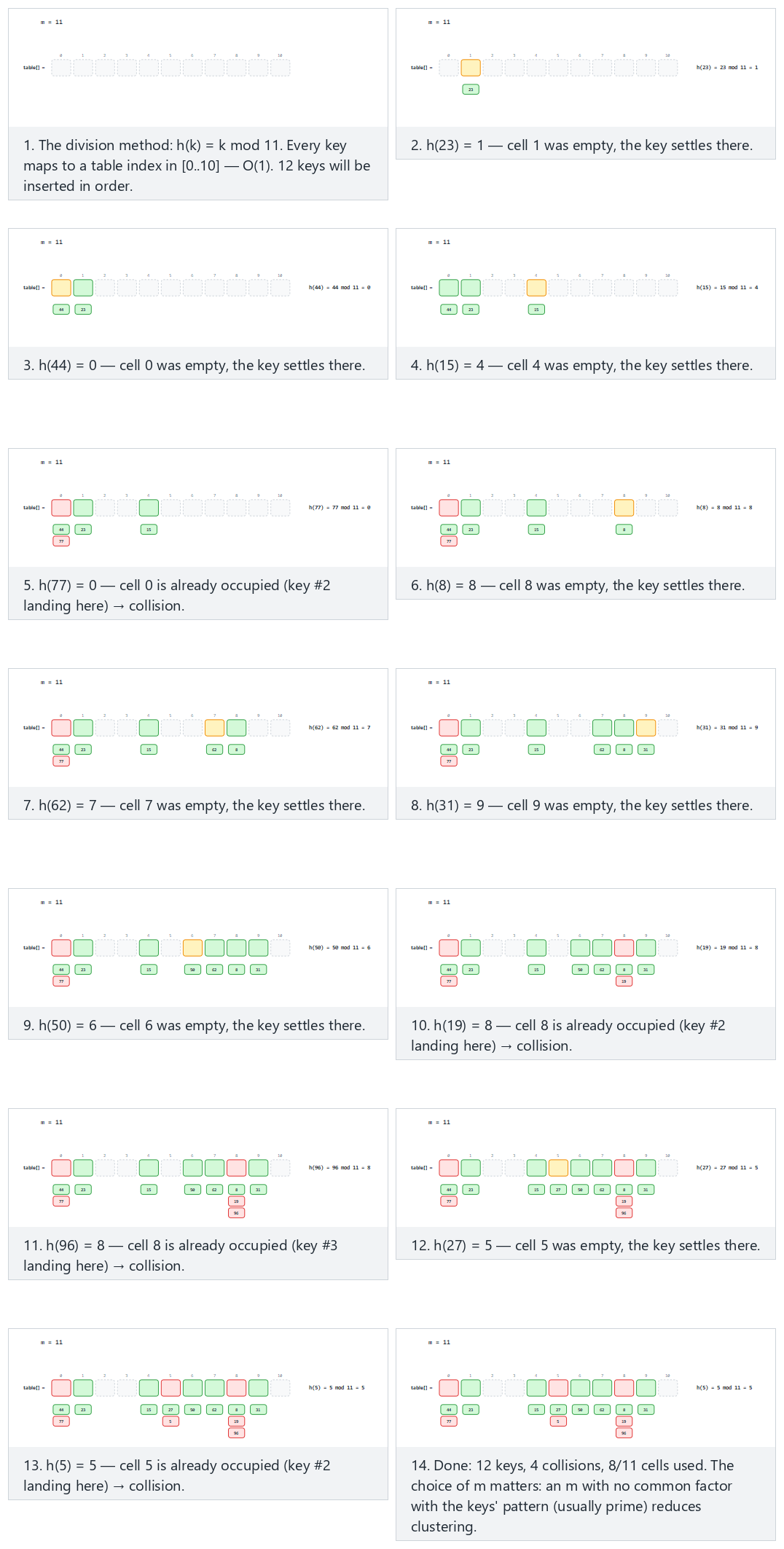
In the picker, also try m = 11 is prime, but the keys are 11 apart: it still collides (hard — a reminder that a prime m helps on average, it is not a magic guarantee against every possible key pattern) and the edge cases m = 10 (a power of 10), keys that are multiples of 10: catastrophic clustering, same keys, m = 13 (prime): perfect spread, and negative keys: without the guard the index would be negative — or press 🎲 for random data, or type your own m and key list.
7.6 Try it
Full program: hash_division.c / HashDivision.java
/* Week 6 -- Search and Hashing
* The division hash function: h(k) = k mod m. Maps any integer key to a
* table index in [0..m-1]. The extra "+ m) % m" guards against negative
* keys. Prints each key's hash and whether it collides with an
* already-occupied bucket.
* CEN207 Data Structures (formerly CE205)
*/
#include <stdio.h>
/* the extra "+ m) % m" guards against negative keys: in C, key % m can be negative when key < 0 */
int hash_division(int key, int m) {
    return ((key % m) + m) % m;
}
static void run_scenario(const char *label, int m, const int keys[], int n) {
printf("-- %s --\n", label);
printf("m = %d\n", m);
int counts[64] = {0};
int collisions = 0;
for (int i = 0; i < n; i++) {
int key = keys[i];
int idx = hash_division(key, m);
int collided = counts[idx] > 0;
if (collided) collisions++;
counts[idx]++;
printf(" h(%d) = %d mod %d = %d%s\n", key, key, m, idx, collided ? " -- collision" : "");
}
int used = 0;
for (int i = 0; i < m; i++) if (counts[i] > 0) used++;
printf("summary: %d keys, %d collisions, %d/%d cells used\n\n", n, collisions, used, m);
}
int main(void) {
int normal[] = {23, 44, 15, 77, 8, 62, 31, 50, 19, 96, 27, 5};
int hard[] = {12, 23, 34, 45, 56, 67, 78, 89, 100, 111, 122, 133, 144};
int power_of_10[] = {10, 20, 30, 40, 50, 60, 70, 80, 90, 100, 110};
int prime_same_keys[] = {10, 20, 30, 40, 50, 60, 70, 80, 90, 100, 110};
int negative_keys[] = {-3, -15, -27, 5, 18, -42, 33, -8, 50, -19, 7};
run_scenario("normal: m = 11 (prime), 12 assorted keys", 11, normal, 12);
run_scenario("hard: m = 11 is prime, but the keys are 11 apart: it still collides", 11, hard, 13);
run_scenario("edge: m = 10 (a power of 10), keys that are multiples of 10: catastrophic clustering", 10, power_of_10, 11);
run_scenario("edge: same keys, m = 13 (prime): perfect spread", 13, prime_same_keys, 11);
run_scenario("edge: negative keys, without the guard the index would be negative", 11, negative_keys, 11);
return 0;
}
/* Week 6 -- Search and Hashing
* The division hash function: h(k) = k mod m. Maps any integer key to a
* table index in [0..m-1]. The extra "+ m) % m" guards against negative
* keys. Prints each key's hash and whether it collides with an
* already-occupied bucket.
* CEN207 Data Structures (formerly CE205)
*/
public class HashDivision {
// the extra "+ m) % m" guards against negative keys: in Java, key % m can be negative when key < 0
static int hashDivision(int key, int m) {
    return ((key % m) + m) % m;
}
static void runScenario(String label, int m, int[] keys) {
System.out.println("-- " + label + " --");
System.out.println("m = " + m);
int[] counts = new int[64];
int collisions = 0;
for (int key : keys) {
int idx = hashDivision(key, m);
boolean collided = counts[idx] > 0;
if (collided) collisions++;
counts[idx]++;
System.out.println(" h(" + key + ") = " + key + " mod " + m + " = " + idx + (collided ? " -- collision" : ""));
}
int used = 0;
for (int i = 0; i < m; i++) if (counts[i] > 0) used++;
System.out.println("summary: " + keys.length + " keys, " + collisions + " collisions, " + used + "/" + m + " cells used");
System.out.println();
}
public static void main(String[] args) {
int[] normal = {23, 44, 15, 77, 8, 62, 31, 50, 19, 96, 27, 5};
int[] hard = {12, 23, 34, 45, 56, 67, 78, 89, 100, 111, 122, 133, 144};
int[] powerOf10 = {10, 20, 30, 40, 50, 60, 70, 80, 90, 100, 110};
int[] primeSameKeys = {10, 20, 30, 40, 50, 60, 70, 80, 90, 100, 110};
int[] negativeKeys = {-3, -15, -27, 5, 18, -42, 33, -8, 50, -19, 7};
runScenario("normal: m = 11 (prime), 12 assorted keys", 11, normal);
runScenario("hard: m = 11 is prime, but the keys are 11 apart: it still collides", 11, hard);
runScenario("edge: m = 10 (a power of 10), keys that are multiples of 10: catastrophic clustering", 10, powerOf10);
runScenario("edge: same keys, m = 13 (prime): perfect spread", 13, primeSameKeys);
runScenario("edge: negative keys, without the guard the index would be negative", 11, negativeKeys);
}
}
Try it
Expected output:
-- normal: m = 11 (prime), 12 assorted keys --
m = 11
  h(23) = 23 mod 11 = 1
  h(44) = 44 mod 11 = 0
  h(15) = 15 mod 11 = 4
  h(77) = 77 mod 11 = 0 -- collision
  h(8) = 8 mod 11 = 8
  h(62) = 62 mod 11 = 7
  h(31) = 31 mod 11 = 9
  h(50) = 50 mod 11 = 6
  h(19) = 19 mod 11 = 8 -- collision
  h(96) = 96 mod 11 = 8 -- collision
  h(27) = 27 mod 11 = 5
  h(5) = 5 mod 11 = 5 -- collision
summary: 12 keys, 4 collisions, 8/11 cells used

-- hard: m = 11 is prime, but the keys are 11 apart: it still collides --
m = 11
  h(12) = 12 mod 11 = 1
  h(23) = 23 mod 11 = 1 -- collision
  h(34) = 34 mod 11 = 1 -- collision
  h(45) = 45 mod 11 = 1 -- collision
  h(56) = 56 mod 11 = 1 -- collision
  h(67) = 67 mod 11 = 1 -- collision
  h(78) = 78 mod 11 = 1 -- collision
  h(89) = 89 mod 11 = 1 -- collision
  h(100) = 100 mod 11 = 1 -- collision
  h(111) = 111 mod 11 = 1 -- collision
  h(122) = 122 mod 11 = 1 -- collision
  h(133) = 133 mod 11 = 1 -- collision
  h(144) = 144 mod 11 = 1 -- collision
summary: 13 keys, 12 collisions, 1/11 cells used

-- edge: m = 10 (a power of 10), keys that are multiples of 10: catastrophic clustering --
m = 10
  h(10) = 10 mod 10 = 0
  h(20) = 20 mod 10 = 0 -- collision
  h(30) = 30 mod 10 = 0 -- collision
  h(40) = 40 mod 10 = 0 -- collision
  h(50) = 50 mod 10 = 0 -- collision
  h(60) = 60 mod 10 = 0 -- collision
  h(70) = 70 mod 10 = 0 -- collision
  h(80) = 80 mod 10 = 0 -- collision
  h(90) = 90 mod 10 = 0 -- collision
  h(100) = 100 mod 10 = 0 -- collision
  h(110) = 110 mod 10 = 0 -- collision
summary: 11 keys, 10 collisions, 1/10 cells used

-- edge: same keys, m = 13 (prime): perfect spread --
m = 13
  h(10) = 10 mod 13 = 10
  h(20) = 20 mod 13 = 7
  h(30) = 30 mod 13 = 4
  h(40) = 40 mod 13 = 1
  h(50) = 50 mod 13 = 11
  h(60) = 60 mod 13 = 8
  h(70) = 70 mod 13 = 5
  h(80) = 80 mod 13 = 2
  h(90) = 90 mod 13 = 12
  h(100) = 100 mod 13 = 9
  h(110) = 110 mod 13 = 6
summary: 11 keys, 0 collisions, 11/13 cells used

-- edge: negative keys, without the guard the index would be negative --
m = 11
  h(-3) = -3 mod 11 = 8
  h(-15) = -15 mod 11 = 7
  h(-27) = -27 mod 11 = 6
  h(5) = 5 mod 11 = 5
  h(18) = 18 mod 11 = 7 -- collision
  h(-42) = -42 mod 11 = 2
  h(33) = 33 mod 11 = 0
  h(-8) = -8 mod 11 = 3
  h(50) = 50 mod 11 = 6 -- collision
  h(-19) = -19 mod 11 = 3 -- collision
  h(7) = 7 mod 11 = 7 -- collision
summary: 11 keys, 4 collisions, 7/11 cells used
7.7 Complexity, mistakes, self-check
Complexity. Computing h(k) is O(1) — a single modulo operation, regardless of m or how many keys are already in the table. This is the entire appeal of hashing: no comparisons, no narrowing, no dependence on n.
Common mistakes
- Choosing
mas a power of 2 "for speed" (key & (m - 1)instead ofkey % m), without checking the key pattern. This is a completely valid optimization when keys are well-distributed, but the "power of 10, keys that are multiples of 10" scenario above generalizes: a power-of-2mcombined with keys that share low-order bits in common (very common with, say, memory addresses or anything padded/aligned) collides just as catastrophically. - Forgetting the negative-key guard in a language (like C or Java) where
%can return negative results. A hash function that occasionally returns a negative "index" will crash or corrupt memory the first time it is used to index into an actual array. - Treating "
mis prime" as a complete solution to collisions. As the "hard" scenario above shows (m = 11, keys11apart), a primemis a good default heuristic, not a guarantee against every possible key pattern — collisions are always possible and always need a resolution strategy, which is exactly what sections 8 and 9 provide.
Self-check: why does a power-of-10 table size collide so badly?
In the "edge: m = 10" scenario above, every single key collides into index 0. Explain algebraically why key mod 10 is always 0 for every key in that list, and state the general rule this is an example of.
Answer. Every key in that scenario is a multiple of 10 (10, 20, 30, ...), and any multiple of 10, divided by 10, has remainder 0 by definition — so key mod 10 = 0 for all of them. The general rule: if d is a common factor of m and of every key (or of the difference between keys, as in the "hard" scenario where all keys are 11 apart and m = 11), then those keys collide. Choosing m prime, with no common factors with typical key patterns, minimizes (but never fully eliminates) this risk.
8. Collisions and separate chaining
8.1 A question to start
Section 7 ended on a fact you cannot design your way out of: two different keys can hash to the same index. Even with m chosen carefully, the moment you insert more keys than there are slots (or just get unlucky), a collision will happen. Once h(key1) == h(key2) for two different keys, both cannot occupy the same single array slot — so what happens to the second one? The simplest possible answer: don't make the slot hold one key — make it hold a list of every key that ever hashed there.
8.2 The idea: one linked list per slot
Separate chaining (sometimes called "closed addressing", though "chaining" is the more common name) gives every table slot a linked list — a chain — of every key that has hashed to it. Inserting a key computes h(key) and adds a new node to the head of that slot's chain — an O(1) operation, exactly like the head-insertion you learned in Week 2. A collision no longer overwrites anything or needs any special handling at insert time; it simply means the chain at that slot now has two (or more) nodes. Searching for a key computes h(key) and then walks that one chain — and only that chain, never any other slot's — comparing each node's key until a match is found or the chain ends.
8.3 Load factor: how "full" is the table, really?
Because chaining never runs out of room (a chain can always grow one more node), the notion of a hash table being "full" does not really apply the way it does for a plain array. Instead, chaining is measured by the load factor, alpha = n / m — the number of keys n divided by the number of slots m — which is the average chain length. A search that misses (the key is not in the table) must, on average, walk the entire average chain before concluding that: O(1 + alpha). When alpha is kept small (a small, constant number of keys per slot on average, by growing the table as it fills — section 10's rehashing), this stays close to O(1). When alpha grows large (many keys crammed behind a small m, as in the "high load" and "single bucket" scenarios you will run below), search degrades toward the O(n) of a single very long linked list.
8.4 In memory, and the code
typedef struct Node { int key; struct Node *next; } Node;
Node *table[M];                       /* M buckets, each the head of a chain (NULL = empty) */

void insert(int key) {
    int idx = key % M;
    Node *n = malloc(sizeof(Node));
    n->key = key;
    n->next = table[idx];              /* new node becomes the head: O(1) */
    table[idx] = n;
}

bool search(int key, int *probes) {
    int idx = key % M;
    int p = 0;
    for (Node *cur = table[idx]; cur != NULL; cur = cur->next) {
        p++;
        if (cur->key == key) { *probes = p; return true; }
    }
    *probes = p;
    return false;
}
static class Node { int key; Node next; Node(int k, Node nx) { key = k; next = nx; } }
Node[] table = new Node[M];            // M buckets, each the head of a chain (null = empty)

void insert(int key) {
    int idx = key % M;
    table[idx] = new Node(key, table[idx]);   // new node becomes the head: O(1)
}

boolean search(int key) {
    int idx = key % M;
    probes = 0;
    for (Node cur = table[idx]; cur != null; cur = cur.next) {
        probes++;
        if (cur.key == key) return true;
    }
    return false;
}
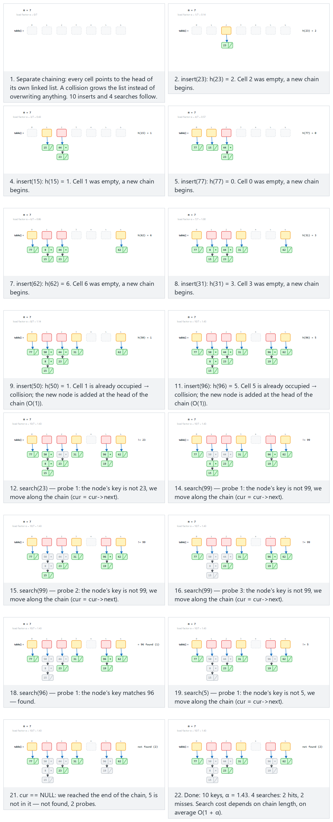
In the picker, also try m = 5, 12 inserts: chains grow, 5 searches (hard) and the edge cases m = 1: every key in one chain, search degrades to O(n) and m = 3, 12 keys: load factor α = 4 — or press 🎲 for random data, or type your own m plus a mix of inserts and search=N queries.
8.5 Try it
Full program: hash_chaining.c / HashChaining.java
/* Week 6 -- Search and Hashing
 * Hash table with separate chaining: each bucket holds the head of a linked
 * list ("chain") of every key that hashed there. A collision grows the
 * chain instead of overwriting anything. Insertion is O(1); search walks
 * the chain, so its cost depends on the chain's length.
 * CEN207 Data Structures (formerly CE205)
 */
#include <stdio.h>
#include <stdlib.h>

#define MAX_M 16

typedef struct Node { int key; struct Node *next; } Node;
Node *table[MAX_M];                    /* M buckets, each the head of a chain (NULL = empty) */
int M;

static int h(int key) { return ((key % M) + M) % M; }

void insert(int key) {
    int idx = h(key);
    Node *n = malloc(sizeof(Node));
    n->key = key;
    n->next = table[idx];              /* new node becomes the head: O(1) */
    table[idx] = n;
}

int search(int key, int *probes) {
    int idx = h(key);
    int p = 0;
    for (Node *cur = table[idx]; cur != NULL; cur = cur->next) {
        p++;
        if (cur->key == key) { *probes = p; return 1; }
    }
    *probes = p;
    return 0;
}

static void clear_table(void) {
    for (int i = 0; i < MAX_M; i++) {
        Node *cur = table[i];
        while (cur) { Node *nx = cur->next; free(cur); cur = nx; }
        table[i] = NULL;
    }
}

typedef struct { int is_search; int value; } Op;

static void run_scenario(const char *label, int m, Op ops[], int n) {
    printf("-- %s --\n", label);
    printf("m = %d\n", m);
    M = m;
    clear_table();
    int inserted = 0;
    for (int i = 0; i < n; i++) {
        if (!ops[i].is_search) {
            int key = ops[i].value;
            int idx = h(key);
            int collided = table[idx] != NULL;
            insert(key);
            inserted++;
            printf("  insert(%d): h(%d) = %d%s (load factor alpha = %d/%d = %.2f)\n",
                   key, key, idx, collided ? " -- collision, added at head of chain" : " -- empty bucket, new chain",
                   inserted, m, (double) inserted / m);
        } else {
            int key = ops[i].value;
            int probes = 0;
            int found = search(key, &probes);
            printf("  search(%d): h(%d) = %d -- %s, %d probes\n",
                   key, key, h(key), found ? "found" : "not found", probes);
        }
    }
    printf("summary: %d keys inserted, load factor alpha = %.2f\n\n", inserted, (double) inserted / m);
    clear_table();
}

int main(void) {
    Op normal[] = {
        {0, 23}, {0, 44}, {0, 15}, {0, 77}, {0, 8}, {0, 62}, {0, 31}, {0, 50}, {0, 19}, {0, 96},
        {1, 23}, {1, 99}, {1, 96}, {1, 5}
    };
    Op hard[] = {
        {0, 12}, {0, 27}, {0, 42}, {0, 7}, {0, 33}, {0, 18}, {0, 53}, {0, 9}, {0, 44}, {0, 21}, {0, 38}, {0, 16},
        {1, 12}, {1, 100}, {1, 16}, {1, 61}, {1, 9}
    };
    Op single_bucket[] = {
        {0, 5}, {0, 17}, {0, 29}, {0, 3}, {0, 41}, {0, 12}, {0, 8}, {0, 50}, {0, 23}, {0, 36},
        {1, 36}, {1, 99}
    };
    Op high_load[] = {
        {0, 4}, {0, 10}, {0, 16}, {0, 22}, {0, 28}, {0, 34}, {0, 40}, {0, 46}, {0, 52}, {0, 58}, {0, 64}, {0, 70},
        {1, 58}, {1, 100}, {1, 4}
    };

    run_scenario("normal: m = 7, 10 inserts, 4 searches (hits and misses)", 7, normal, 14);
    run_scenario("hard: m = 5, 12 inserts: chains grow, 5 searches", 5, hard, 17);
    run_scenario("edge: m = 1, every key in one chain, search degrades to O(n)", 1, single_bucket, 12);
    run_scenario("edge: m = 3, 12 keys: load factor alpha = 4", 3, high_load, 15);

    return 0;
}
/* Week 6 -- Search and Hashing
 * Hash table with separate chaining: each bucket holds the head of a linked
 * list ("chain") of every key that hashed there. A collision grows the
 * chain instead of overwriting anything. Insertion is O(1); search walks
 * the chain, so its cost depends on the chain's length.
 * CEN207 Data Structures (formerly CE205)
 */
public class HashChaining {
    static class Node { int key; Node next; Node(int k, Node nx) { key = k; next = nx; } }

    static final int MAX_M = 16;
    static Node[] table = new Node[MAX_M];
    static int m;

    static int h(int key) { return ((key % m) + m) % m; }

    static void insert(int key) {
        int idx = h(key);
        table[idx] = new Node(key, table[idx]);   // new node becomes the head: O(1)
    }

    static int probesUsed;
    static boolean search(int key) {
        int idx = h(key);
        probesUsed = 0;
        for (Node cur = table[idx]; cur != null; cur = cur.next) {
            probesUsed++;
            if (cur.key == key) return true;
        }
        return false;
    }

    static void clearTable() { for (int i = 0; i < MAX_M; i++) table[i] = null; }

    static class Op { boolean isSearch; int value; Op(boolean s, int v) { isSearch = s; value = v; } }

    static void runScenario(String label, int mm, Op[] ops) {
        System.out.println("-- " + label + " --");
        System.out.println("m = " + mm);
        m = mm;
        clearTable();
        int inserted = 0;
        for (Op op : ops) {
            if (!op.isSearch) {
                int key = op.value;
                int idx = h(key);
                boolean collided = table[idx] != null;
                insert(key);
                inserted++;
                System.out.println("  insert(" + key + "): h(" + key + ") = " + idx
                        + (collided ? " -- collision, added at head of chain" : " -- empty bucket, new chain")
                        + " (load factor alpha = " + inserted + "/" + m + " = " + String.format("%.2f", (double) inserted / m) + ")");
            } else {
                int key = op.value;
                boolean found = search(key);
                System.out.println("  search(" + key + "): h(" + key + ") = " + h(key) + " -- " + (found ? "found" : "not found") + ", " + probesUsed + " probes");
            }
        }
        System.out.println("summary: " + inserted + " keys inserted, load factor alpha = " + String.format("%.2f", (double) inserted / m));
        System.out.println();
        clearTable();
    }

    public static void main(String[] args) {
        Op[] normal = {
            new Op(false, 23), new Op(false, 44), new Op(false, 15), new Op(false, 77), new Op(false, 8),
            new Op(false, 62), new Op(false, 31), new Op(false, 50), new Op(false, 19), new Op(false, 96),
            new Op(true, 23), new Op(true, 99), new Op(true, 96), new Op(true, 5)
        };
        Op[] hard = {
            new Op(false, 12), new Op(false, 27), new Op(false, 42), new Op(false, 7), new Op(false, 33),
            new Op(false, 18), new Op(false, 53), new Op(false, 9), new Op(false, 44), new Op(false, 21),
            new Op(false, 38), new Op(false, 16),
            new Op(true, 12), new Op(true, 100), new Op(true, 16), new Op(true, 61), new Op(true, 9)
        };
        Op[] singleBucket = {
            new Op(false, 5), new Op(false, 17), new Op(false, 29), new Op(false, 3), new Op(false, 41),
            new Op(false, 12), new Op(false, 8), new Op(false, 50), new Op(false, 23), new Op(false, 36),
            new Op(true, 36), new Op(true, 99)
        };
        Op[] highLoad = {
            new Op(false, 4), new Op(false, 10), new Op(false, 16), new Op(false, 22), new Op(false, 28),
            new Op(false, 34), new Op(false, 40), new Op(false, 46), new Op(false, 52), new Op(false, 58),
            new Op(false, 64), new Op(false, 70),
            new Op(true, 58), new Op(true, 100), new Op(true, 4)
        };

        runScenario("normal: m = 7, 10 inserts, 4 searches (hits and misses)", 7, normal);
        runScenario("hard: m = 5, 12 inserts: chains grow, 5 searches", 5, hard);
        runScenario("edge: m = 1, every key in one chain, search degrades to O(n)", 1, singleBucket);
        runScenario("edge: m = 3, 12 keys: load factor alpha = 4", 3, highLoad);
    }
}
Try it
Expected output:
-- normal: m = 7, 10 inserts, 4 searches (hits and misses) --
m = 7
  insert(23): h(23) = 2 -- empty bucket, new chain (load factor alpha = 1/7 = 0.14)
  insert(44): h(44) = 2 -- collision, added at head of chain (load factor alpha = 2/7 = 0.29)
  insert(15): h(15) = 1 -- empty bucket, new chain (load factor alpha = 3/7 = 0.43)
  insert(77): h(77) = 0 -- empty bucket, new chain (load factor alpha = 4/7 = 0.57)
  insert(8): h(8) = 1 -- collision, added at head of chain (load factor alpha = 5/7 = 0.71)
  insert(62): h(62) = 6 -- empty bucket, new chain (load factor alpha = 6/7 = 0.86)
  insert(31): h(31) = 3 -- empty bucket, new chain (load factor alpha = 7/7 = 1.00)
  insert(50): h(50) = 1 -- collision, added at head of chain (load factor alpha = 8/7 = 1.14)
  insert(19): h(19) = 5 -- empty bucket, new chain (load factor alpha = 9/7 = 1.29)
  insert(96): h(96) = 5 -- collision, added at head of chain (load factor alpha = 10/7 = 1.43)
  search(23): h(23) = 2 -- found, 2 probes
  search(99): h(99) = 1 -- not found, 3 probes
  search(96): h(96) = 5 -- found, 1 probes
  search(5): h(5) = 5 -- not found, 2 probes
summary: 10 keys inserted, load factor alpha = 1.43

-- hard: m = 5, 12 inserts: chains grow, 5 searches --
m = 5
  insert(12): h(12) = 2 -- empty bucket, new chain (load factor alpha = 1/5 = 0.20)
  insert(27): h(27) = 2 -- collision, added at head of chain (load factor alpha = 2/5 = 0.40)
  insert(42): h(42) = 2 -- collision, added at head of chain (load factor alpha = 3/5 = 0.60)
  insert(7): h(7) = 2 -- collision, added at head of chain (load factor alpha = 4/5 = 0.80)
  insert(33): h(33) = 3 -- empty bucket, new chain (load factor alpha = 5/5 = 1.00)
  insert(18): h(18) = 3 -- collision, added at head of chain (load factor alpha = 6/5 = 1.20)
  insert(53): h(53) = 3 -- collision, added at head of chain (load factor alpha = 7/5 = 1.40)
  insert(9): h(9) = 4 -- empty bucket, new chain (load factor alpha = 8/5 = 1.60)
  insert(44): h(44) = 4 -- collision, added at head of chain (load factor alpha = 9/5 = 1.80)
  insert(21): h(21) = 1 -- empty bucket, new chain (load factor alpha = 10/5 = 2.00)
  insert(38): h(38) = 3 -- collision, added at head of chain (load factor alpha = 11/5 = 2.20)
  insert(16): h(16) = 1 -- collision, added at head of chain (load factor alpha = 12/5 = 2.40)
  search(12): h(12) = 2 -- found, 4 probes
  search(100): h(100) = 0 -- not found, 0 probes
  search(16): h(16) = 1 -- found, 1 probes
  search(61): h(61) = 1 -- not found, 2 probes
  search(9): h(9) = 4 -- found, 2 probes
summary: 12 keys inserted, load factor alpha = 2.40

-- edge: m = 1, every key in one chain, search degrades to O(n) --
m = 1
  insert(5): h(5) = 0 -- empty bucket, new chain (load factor alpha = 1/1 = 1.00)
  insert(17): h(17) = 0 -- collision, added at head of chain (load factor alpha = 2/1 = 2.00)
  insert(29): h(29) = 0 -- collision, added at head of chain (load factor alpha = 3/1 = 3.00)
  insert(3): h(3) = 0 -- collision, added at head of chain (load factor alpha = 4/1 = 4.00)
  insert(41): h(41) = 0 -- collision, added at head of chain (load factor alpha = 5/1 = 5.00)
  insert(12): h(12) = 0 -- collision, added at head of chain (load factor alpha = 6/1 = 6.00)
  insert(8): h(8) = 0 -- collision, added at head of chain (load factor alpha = 7/1 = 7.00)
  insert(50): h(50) = 0 -- collision, added at head of chain (load factor alpha = 8/1 = 8.00)
  insert(23): h(23) = 0 -- collision, added at head of chain (load factor alpha = 9/1 = 9.00)
  insert(36): h(36) = 0 -- collision, added at head of chain (load factor alpha = 10/1 = 10.00)
  search(36): h(36) = 0 -- found, 1 probes
  search(99): h(99) = 0 -- not found, 10 probes
summary: 10 keys inserted, load factor alpha = 10.00

-- edge: m = 3, 12 keys: load factor alpha = 4 --
m = 3
  insert(4): h(4) = 1 -- empty bucket, new chain (load factor alpha = 1/3 = 0.33)
  insert(10): h(10) = 1 -- collision, added at head of chain (load factor alpha = 2/3 = 0.67)
  insert(16): h(16) = 1 -- collision, added at head of chain (load factor alpha = 3/3 = 1.00)
  insert(22): h(22) = 1 -- collision, added at head of chain (load factor alpha = 4/3 = 1.33)
  insert(28): h(28) = 1 -- collision, added at head of chain (load factor alpha = 5/3 = 1.67)
  insert(34): h(34) = 1 -- collision, added at head of chain (load factor alpha = 6/3 = 2.00)
  insert(40): h(40) = 1 -- collision, added at head of chain (load factor alpha = 7/3 = 2.33)
  insert(46): h(46) = 1 -- collision, added at head of chain (load factor alpha = 8/3 = 2.67)
  insert(52): h(52) = 1 -- collision, added at head of chain (load factor alpha = 9/3 = 3.00)
  insert(58): h(58) = 1 -- collision, added at head of chain (load factor alpha = 10/3 = 3.33)
  insert(64): h(64) = 1 -- collision, added at head of chain (load factor alpha = 11/3 = 3.67)
  insert(70): h(70) = 1 -- collision, added at head of chain (load factor alpha = 12/3 = 4.00)
  search(58): h(58) = 1 -- found, 3 probes
  search(100): h(100) = 1 -- not found, 12 probes
  search(4): h(4) = 1 -- found, 12 probes
summary: 12 keys inserted, load factor alpha = 4.00
8.6 Complexity, mistakes, self-check
Complexity. Insert: O(1) always (head insertion never needs to walk the chain). Search (and delete, which is not shown above but works the same way): O(1 + alpha) on average, where alpha = n/m is the load factor — the 1 accounts for computing the hash itself, and alpha for the average chain length walked. When alpha is kept bounded by a constant (by growing m as n grows — rehashing, section 10), this is O(1) amortized; when m stays fixed while n grows without bound (as in the "single bucket" and "high load" scenarios above), it degrades toward O(n).
Common mistakes
- Inserting at the tail instead of the head of the chain. Head insertion is O(1) because you already have a pointer to the current head (
table[idx]); tail insertion needs to walk the whole chain first to find its end, turning every insert into an O(chain length) operation for no benefit. - Forgetting to free every node in every chain when a table is discarded (C only). Each chain is a separate linked list — freeing
table[idx]itself is not enough; every node in every chain must be freed individually, exactly as you learned for ordinary linked lists in Week 2. - Assuming a "not found" search is cheap. A search that misses walks the entire chain (there is no early exit except reaching the end) — on a table with a high load factor, a miss can be just as expensive as, or more expensive than, a hit deep in a chain.
Self-check: load factor and search cost
In the "m = 1" scenario above, every one of the 10 keys hashes to the same single bucket. What is the load factor alpha after all 10 inserts, and why does search(99) (a miss) need exactly 10 probes while search(36) (the most recently inserted key) needs only 1?
Answer. alpha = n/m = 10/1 = 10.00 — the single chain holds all 10 keys. search(36) finds it immediately because it was the last key inserted, and insertion always adds at the head of the chain — so the most recently inserted key is always the cheapest to find. search(99) is a miss: since 99 is nowhere in the chain, the search must walk every single node, from head to the end (NULL/null), before it can conclude "not found" — all 10 probes, confirming the O(1 + alpha) cost with alpha = 10.
9. Open addressing: linear probing, quadratic probing, double hashing
Separate chaining solves collisions by growing a second structure (a linked list) hanging off each table slot. Open addressing takes the opposite approach: every key lives directly inside the table array itself, no linked lists at all. On a collision, the algorithm probes — tries another slot, following some fixed rule — until it finds an empty one. The three probing rules below differ only in which slot they try next.
9.1 Linear probing
9.1.1 A question to start
The simplest possible probing rule: if the home slot h(key) is occupied, try the very next slot, h(key) + 1; if that is occupied too, try h(key) + 2; and so on, wrapping around to the start of the table if you fall off the end. This is linear probing.
9.1.2 Insert, search, and the tombstone problem
Each slot needs a small piece of state beyond just its key: EMPTY (never used), OCCUPIED (holds a key), or DELETED. Insert probes from h(key) until it finds a slot that is EMPTY or DELETED — either can be reused — and places the key there. Search probes from h(key) and stops the instant it hits an EMPTY slot (sorted-search logic does not apply here, but the same "no need to look further" idea does: if the slot were ever occupied by this key, it would have been placed no later than the first empty slot encountered during its own insertion) — but it must keep going past a DELETED slot, not stop there, because a DELETED slot only means "a key that once probed through here was removed", not "no key past this point exists". Delete does not simply mark a slot EMPTY — doing so would silently break the probe chain for every key that was inserted after it and had to probe past it. Instead, delete leaves a tombstone: the slot becomes DELETED, which search treats as "occupied, keep probing" and insert treats as "free, reusable".
9.1.3 Primary clustering
Linear probing's weakness is primary clustering: once several keys collide near each other, the occupied run of slots grows, and a longer occupied run is more likely to catch the next colliding key too (more consecutive slots for a probe sequence to land inside), making the run grow even longer still. This snowballing effect is visible directly in the animation below as a cluster of neighbouring filled cells.
9.1.4 In memory, and the code
typedef enum { EMPTY, OCCUPIED, DELETED } Slot;
Slot state[M];                        /* all EMPTY initially */
int table[M];

bool insert(int key) {
    int idx = key % M;
    for (int i = 0; i < M; i++) {
        if (state[idx] != OCCUPIED) {          /* EMPTY or DELETED: reuse this slot */
            table[idx] = key;
            state[idx] = OCCUPIED;
            return true;
        }
        idx = (idx + 1) % M;                   /* linear probing: try the next slot */
    }
    return false;                              /* table full: M slots probed, none free */
}

bool search(int key, int *probes) {
    int idx = key % M, p = 0;
    for (int i = 0; i < M; i++) {
        p++;
        if (state[idx] == EMPTY) { *probes = p; return false; }   /* gap: key cannot be further */
        if (state[idx] == OCCUPIED && table[idx] == key) { *probes = p; return true; }
        idx = (idx + 1) % M;
    }
    *probes = p;
    return false;
}

bool delete_key(int key) {
    int idx = key % M;
    for (int i = 0; i < M; i++) {
        if (state[idx] == EMPTY) return false;
        if (state[idx] == OCCUPIED && table[idx] == key) { state[idx] = DELETED; return true; }
        idx = (idx + 1) % M;
    }
    return false;
}
static final int EMPTY = 0, OCCUPIED = 1, DELETED = 2;
int[] state = new int[M];              // all EMPTY (0) initially
int[] table = new int[M];

boolean insert(int key) {
    int idx = key % M;
    for (int i = 0; i < M; i++) {
        if (state[idx] != OCCUPIED) {          // EMPTY or DELETED: reuse this slot
            table[idx] = key;
            state[idx] = OCCUPIED;
            return true;
        }
        idx = (idx + 1) % M;                   // linear probing: try the next slot
    }
    return false;                              // table full: M slots probed, none free
}

boolean search(int key) {
    int idx = key % M;
    probes = 0;
    for (int i = 0; i < M; i++) {
        probes++;
        if (state[idx] == EMPTY) return false;   // gap: key cannot be further
        if (state[idx] == OCCUPIED && table[idx] == key) return true;
        idx = (idx + 1) % M;
    }
    return false;
}

boolean deleteKey(int key) {
    int idx = key % M;
    for (int i = 0; i < M; i++) {
        if (state[idx] == EMPTY) return false;
        if (state[idx] == OCCUPIED && table[idx] == key) { state[idx] = DELETED; return true; }
        idx = (idx + 1) % M;
    }
    return false;
}
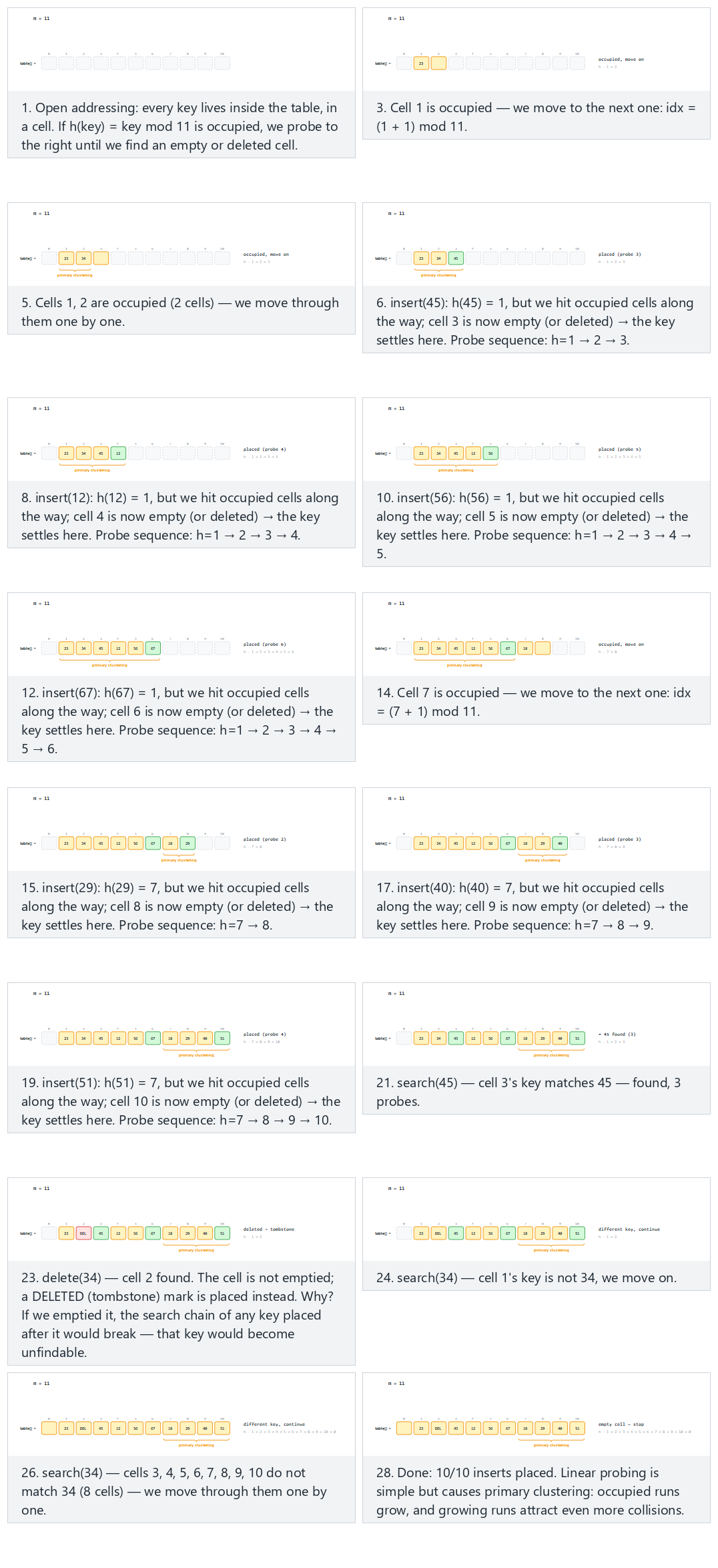
In the picker, also try m = 11, the keys collide into two big clusters (hard) and the edge cases m = 8, 8 keys into the same cell: the table fills exactly, later inserts are rejected and search after a delete: why it would go wrong without a tombstone — or press 🎲 for random data, or type your own m plus a mix of inserts, search=N, and del=N.
9.1.5 Try it
Full program: hash_linear_probing.c / HashLinearProbing.java
/* Week 6 -- Search and Hashing
 * Open addressing with linear probing: every key lives directly IN the
 * table. On a collision, probe the next slot, wrapping around, until an
 * empty (or deleted) slot is found. A deleted slot gets a tombstone marker,
 * not a plain empty mark, so search keeps walking past it.
 * CEN207 Data Structures (formerly CE205)
 */
#include <stdio.h>

#define MAX_M 16
typedef enum { EMPTY, OCCUPIED, DELETED } Slot;
Slot state[MAX_M];
int table[MAX_M];
int M;

static int h(int key) { return ((key % M) + M) % M; }

int insert(int key, int *probes) {
    int idx = h(key);
    for (int i = 0; i < M; i++) {
        (*probes)++;
        if (state[idx] != OCCUPIED) {          /* EMPTY or DELETED: reuse this slot */
            table[idx] = key;
            state[idx] = OCCUPIED;
            return idx;
        }
        idx = (idx + 1) % M;                   /* linear probing: try the next slot */
    }
    return -1;                              /* table full: M slots probed, none free */
}

int search(int key, int *probes) {
    int idx = h(key);
    for (int i = 0; i < M; i++) {
        (*probes)++;
        if (state[idx] == EMPTY) return -1;   /* gap: key cannot be further */
        if (state[idx] == OCCUPIED && table[idx] == key) return idx;
        idx = (idx + 1) % M;
    }
    return -1;
}

int delete_key(int key, int *probes) {
    int idx = h(key);
    for (int i = 0; i < M; i++) {
        (*probes)++;
        if (state[idx] == EMPTY) return -1;
        if (state[idx] == OCCUPIED && table[idx] == key) { state[idx] = DELETED; return idx; }
        idx = (idx + 1) % M;
    }
    return -1;
}

typedef struct { int kind; int value; } Op;   /* kind: 0 insert, 1 search, 2 delete */

static void clear_table(void) { for (int i = 0; i < MAX_M; i++) { state[i] = EMPTY; table[i] = 0; } }

static void run_scenario(const char *label, int m, Op ops[], int n) {
    printf("-- %s --\n", label);
    printf("m = %d\n", m);
    M = m;
    clear_table();
    int placed_count = 0, rejected = 0;
    for (int i = 0; i < n; i++) {
        int probes = 0;
        if (ops[i].kind == 0) {
            int key = ops[i].value;
            int idx = insert(key, &probes);
            if (idx == -1) { rejected++; printf("  insert(%d): table full, rejected (%d probes)\n", key, probes); }
            else { placed_count++; printf("  insert(%d): placed at %d (%d probe%s)\n", key, idx, probes, probes == 1 ? "" : "s"); }
        } else if (ops[i].kind == 1) {
            int key = ops[i].value;
            int idx = search(key, &probes);
            printf("  search(%d): %s (%d probes)\n", key, idx == -1 ? "not found" : "found", probes);
        } else {
            int key = ops[i].value;
            int idx = delete_key(key, &probes);
            printf("  delete(%d): %s (%d probes)\n", key, idx == -1 ? "not found" : "deleted, tombstone left", probes);
        }
    }
    printf("summary: %d/%d inserts placed%s\n\n", placed_count, placed_count + rejected,
           rejected ? " (table full for the rest)" : "");
}

int main(void) {
    Op normal[] = {
        {0, 23}, {0, 34}, {0, 45}, {0, 12}, {0, 56}, {0, 67}, {0, 18}, {0, 29}, {0, 40}, {0, 51},
        {1, 45}, {2, 34}, {1, 34}
    };
    Op hard[] = {
        {0, 11}, {0, 22}, {0, 33}, {0, 44}, {0, 55}, {0, 5}, {0, 16}, {0, 27}, {0, 38}, {0, 49},
        {1, 49}, {2, 22}, {1, 33}, {1, 22}
    };
    Op table_full[] = {
        {0, 3}, {0, 11}, {0, 19}, {0, 27}, {0, 35}, {0, 43}, {0, 51}, {0, 59}, {0, 99}, {0, 67}
    };
    Op tombstone[] = {
        {0, 15}, {0, 26}, {0, 37}, {0, 8}, {0, 19}, {0, 30}, {0, 41}, {0, 52}, {0, 63}, {0, 74},
        {2, 26}, {1, 37}, {1, 26}
    };

    run_scenario("normal: m = 11, 10 inserts, a search and a delete", 11, normal, 13);
    run_scenario("hard: m = 11, the keys collide into two big clusters", 11, hard, 14);
    run_scenario("edge: m = 8, 8 keys into the same cell: the table fills exactly, later inserts are rejected", 8, table_full, 10);
    run_scenario("edge: search after a delete, why it would go wrong without a tombstone", 11, tombstone, 13);

    return 0;
}
/* Week 6 -- Search and Hashing
 * Open addressing with linear probing: every key lives directly IN the
 * table. On a collision, probe the next slot, wrapping around, until an
 * empty (or deleted) slot is found. A deleted slot gets a tombstone marker,
 * not a plain empty mark, so search keeps walking past it.
 * CEN207 Data Structures (formerly CE205)
 */
public class HashLinearProbing {
    static final int EMPTY = 0, OCCUPIED = 1, DELETED = 2;
    static final int MAX_M = 16;
    static int[] state = new int[MAX_M];
    static int[] table = new int[MAX_M];
    static int m;

    static int h(int key) { return ((key % m) + m) % m; }

    static int probes;

    static int insert(int key) {
        int idx = h(key);
        for (int i = 0; i < m; i++) {
            probes++;
            if (state[idx] != OCCUPIED) {          // EMPTY or DELETED: reuse this slot
                table[idx] = key;
                state[idx] = OCCUPIED;
                return idx;
            }
            idx = (idx + 1) % m;                   // linear probing: try the next slot
        }
        return -1;                              // table full: m slots probed, none free
    }

    static int search(int key) {
        int idx = h(key);
        for (int i = 0; i < m; i++) {
            probes++;
            if (state[idx] == EMPTY) return -1;   // gap: key cannot be further
            if (state[idx] == OCCUPIED && table[idx] == key) return idx;
            idx = (idx + 1) % m;
        }
        return -1;
    }

    static int deleteKey(int key) {
        int idx = h(key);
        for (int i = 0; i < m; i++) {
            probes++;
            if (state[idx] == EMPTY) return -1;
            if (state[idx] == OCCUPIED && table[idx] == key) { state[idx] = DELETED; return idx; }
            idx = (idx + 1) % m;
        }
        return -1;
    }

    static class Op { int kind; int value; Op(int k, int v) { kind = k; value = v; } }  // kind: 0 insert, 1 search, 2 delete

    static void clearTable() { for (int i = 0; i < MAX_M; i++) { state[i] = EMPTY; table[i] = 0; } }

    static void runScenario(String label, int mm, Op[] ops) {
        System.out.println("-- " + label + " --");
        System.out.println("m = " + mm);
        m = mm;
        clearTable();
        int placedCount = 0, rejected = 0;
        for (Op op : ops) {
            probes = 0;
            if (op.kind == 0) {
                int key = op.value;
                int idx = insert(key);
                if (idx == -1) { rejected++; System.out.println("  insert(" + key + "): table full, rejected (" + probes + " probes)"); }
                else { placedCount++; System.out.println("  insert(" + key + "): placed at " + idx + " (" + probes + " probe" + (probes == 1 ? "" : "s") + ")"); }
            } else if (op.kind == 1) {
                int key = op.value;
                int idx = search(key);
                System.out.println("  search(" + key + "): " + (idx == -1 ? "not found" : "found") + " (" + probes + " probes)");
            } else {
                int key = op.value;
                int idx = deleteKey(key);
                System.out.println("  delete(" + key + "): " + (idx == -1 ? "not found" : "deleted, tombstone left") + " (" + probes + " probes)");
            }
        }
        System.out.println("summary: " + placedCount + "/" + (placedCount + rejected) + " inserts placed" + (rejected > 0 ? " (table full for the rest)" : ""));
        System.out.println();
    }

    public static void main(String[] args) {
        Op[] normal = {
            new Op(0, 23), new Op(0, 34), new Op(0, 45), new Op(0, 12), new Op(0, 56), new Op(0, 67),
            new Op(0, 18), new Op(0, 29), new Op(0, 40), new Op(0, 51),
            new Op(1, 45), new Op(2, 34), new Op(1, 34)
        };
        Op[] hard = {
            new Op(0, 11), new Op(0, 22), new Op(0, 33), new Op(0, 44), new Op(0, 55), new Op(0, 5),
            new Op(0, 16), new Op(0, 27), new Op(0, 38), new Op(0, 49),
            new Op(1, 49), new Op(2, 22), new Op(1, 33), new Op(1, 22)
        };
        Op[] tableFull = {
            new Op(0, 3), new Op(0, 11), new Op(0, 19), new Op(0, 27), new Op(0, 35), new Op(0, 43),
            new Op(0, 51), new Op(0, 59), new Op(0, 99), new Op(0, 67)
        };
        Op[] tombstone = {
            new Op(0, 15), new Op(0, 26), new Op(0, 37), new Op(0, 8), new Op(0, 19), new Op(0, 30),
            new Op(0, 41), new Op(0, 52), new Op(0, 63), new Op(0, 74),
            new Op(2, 26), new Op(1, 37), new Op(1, 26)
        };

        runScenario("normal: m = 11, 10 inserts, a search and a delete", 11, normal);
        runScenario("hard: m = 11, the keys collide into two big clusters", 11, hard);
        runScenario("edge: m = 8, 8 keys into the same cell: the table fills exactly, later inserts are rejected", 8, tableFull);
        runScenario("edge: search after a delete, why it would go wrong without a tombstone", 11, tombstone);
    }
}
Try it
Expected output:
-- normal: m = 11, 10 inserts, a search and a delete --
m = 11
  insert(23): placed at 1 (1 probe)
  insert(34): placed at 2 (2 probes)
  insert(45): placed at 3 (3 probes)
  insert(12): placed at 4 (4 probes)
  insert(56): placed at 5 (5 probes)
  insert(67): placed at 6 (6 probes)
  insert(18): placed at 7 (1 probe)
  insert(29): placed at 8 (2 probes)
  insert(40): placed at 9 (3 probes)
  insert(51): placed at 10 (4 probes)
  search(45): found (3 probes)
  delete(34): deleted, tombstone left (2 probes)
  search(34): not found (11 probes)
summary: 10/10 inserts placed

-- hard: m = 11, the keys collide into two big clusters --
m = 11
  insert(11): placed at 0 (1 probe)
  insert(22): placed at 1 (2 probes)
  insert(33): placed at 2 (3 probes)
  insert(44): placed at 3 (4 probes)
  insert(55): placed at 4 (5 probes)
  insert(5): placed at 5 (1 probe)
  insert(16): placed at 6 (2 probes)
  insert(27): placed at 7 (3 probes)
  insert(38): placed at 8 (4 probes)
  insert(49): placed at 9 (5 probes)
  search(49): found (5 probes)
  delete(22): deleted, tombstone left (2 probes)
  search(33): found (3 probes)
  search(22): not found (11 probes)
summary: 10/10 inserts placed

-- edge: m = 8, 8 keys into the same cell: the table fills exactly, later inserts are rejected --
m = 8
  insert(3): placed at 3 (1 probe)
  insert(11): placed at 4 (2 probes)
  insert(19): placed at 5 (3 probes)
  insert(27): placed at 6 (4 probes)
  insert(35): placed at 7 (5 probes)
  insert(43): placed at 0 (6 probes)
  insert(51): placed at 1 (7 probes)
  insert(59): placed at 2 (8 probes)
  insert(99): table full, rejected (8 probes)
  insert(67): table full, rejected (8 probes)
summary: 8/10 inserts placed (table full for the rest)

-- edge: search after a delete, why it would go wrong without a tombstone --
m = 11
  insert(15): placed at 4 (1 probe)
  insert(26): placed at 5 (2 probes)
  insert(37): placed at 6 (3 probes)
  insert(8): placed at 8 (1 probe)
  insert(19): placed at 9 (2 probes)
  insert(30): placed at 10 (3 probes)
  insert(41): placed at 0 (4 probes)
  insert(52): placed at 1 (5 probes)
  insert(63): placed at 2 (6 probes)
  insert(74): placed at 3 (7 probes)
  delete(26): deleted, tombstone left (2 probes)
  search(37): found (3 probes)
  search(26): not found (4 probes)
summary: 10/10 inserts placed
9.1.6 Complexity, mistakes, self-check
Complexity. Average case O(1 / (1 - alpha)) for alpha < 1 (this grows sharply as alpha approaches 1 — a table that is 90% full averages around 10 probes per operation, far worse than chaining's O(1 + alpha) at the same load factor). Worst case O(m) — a single operation can probe every slot in the table, as the "table full" scenario above demonstrates. Requires alpha < 1 always (unlike chaining, an open- addressing table has a hard capacity limit).
Common mistakes
- Deleting by marking a slot
EMPTYinstead ofDELETED. As the "tombstone" scenario shows, this silently breaks search for every key that probed past the deleted slot during its own insertion —searchwould incorrectly stop at the now-EMPTYslot and report "not found" for a key that is still genuinely in the table. - Forgetting to wrap the probe index around the end of the table (
idx = (idx + 1) % M). Without the modulo, probing walks off the end of the array instead of wrapping back to slot 0, even though slot 0 might be free. - Not distinguishing "table full" from "key not found" in
insert's return value. Both can look like "the loop finished without success" if you are not careful — the loop must run for at mostMiterations and explicitly signal failure only after trying every slot once.
Self-check: tombstones
In the "search after a delete" scenario above, 26 is deleted and then search(37) still succeeds in 3 probes, and search(26) correctly reports "not found" in 4 probes rather than stopping early. Walk through why both of these are correct, referring to the probe sequence for each key's home slot.
Answer. 37's home slot is 37 mod 11 = 4, which was already occupied by 15 at insertion time, so 37 probed forward to land at slot 6. Deleting 26 (home slot 4, which had also probed forward, to slot 5) turns slot 5 into a tombstone, but slot 6 (where 37 actually lives) is untouched — so search(37) still walks 4 -> 5 -> 6 and finds it, treating the tombstone at 5 as "occupied, keep going" rather than stopping. search(26)'s home slot is also 4; it probes 4 -> 5, finds the tombstone at 5 (not a match, but not empty either, so it keeps going) -> 6 (occupied by 37, not a match) -> 7 (empty — stop): 4 probes, correctly reporting "not found" only once it reaches a genuinely empty slot.
9.2 Quadratic probing
9.2.1 A question to start
Linear probing's primary clustering happens because every colliding key retraces the exact same path — step +1, +1, +1, … — through an already-crowded run of slots. What if, instead, the probe step grew quickly instead of staying fixed at 1? Quadratic probing tries home + 1^2, home + 2^2, home + 3^2, … — 1, 4, 9, 16, … slots away — spreading colliding keys out much faster and avoiding the "long run gets longer" snowball of linear probing.
9.2.2 The idea, and a new trap
insert(key) computes home = h(key) and then, for i = 0, 1, 2, …, tries slot (home + i*i) mod m until an empty one is found. This does avoid primary clustering — but it introduces a different problem. If m is not prime (the classic bad case: m a power of 2), or if the load factor climbs above 0.5, the sequence i*i mod m can start repeating a small set of slots forever, without ever reaching a genuinely free one — even though free slots still exist elsewhere in the table. This is not the same as the table being full; it is a cycle, and the fix is to keep m prime and keep the load factor at or below 0.5.
9.2.3 In memory, and the code
typedef enum { EMPTY, OCCUPIED } Slot;
Slot state[M];                        /* all EMPTY initially */
int table[M];

bool insert(int key) {
    int home = key % M;
    for (int i = 0; i < M; i++) {
        int idx = (home + i * i) % M;          /* quadratic probing: i^2 offsets */
        if (state[idx] != OCCUPIED) {
            table[idx] = key;
            state[idx] = OCCUPIED;
            return true;
        }
    }
    return false;   /* M probes tried: table full, OR (m not prime / alpha > 0.5) the */
                     /* sequence cycled without ever reaching a free slot           */
}
static final int EMPTY = 0, OCCUPIED = 1;
int[] state = new int[M];              // all EMPTY (0) initially
int[] table = new int[M];

boolean insert(int key) {
    int home = key % M;
    for (int i = 0; i < M; i++) {
        int idx = (home + i * i) % M;          // quadratic probing: i^2 offsets
        if (state[idx] != OCCUPIED) {
            table[idx] = key;
            state[idx] = OCCUPIED;
            return true;
        }
    }
    return false;   // M probes tried: table full, OR (m not prime / alpha > 0.5) the
                    // sequence cycled without ever reaching a free slot
}
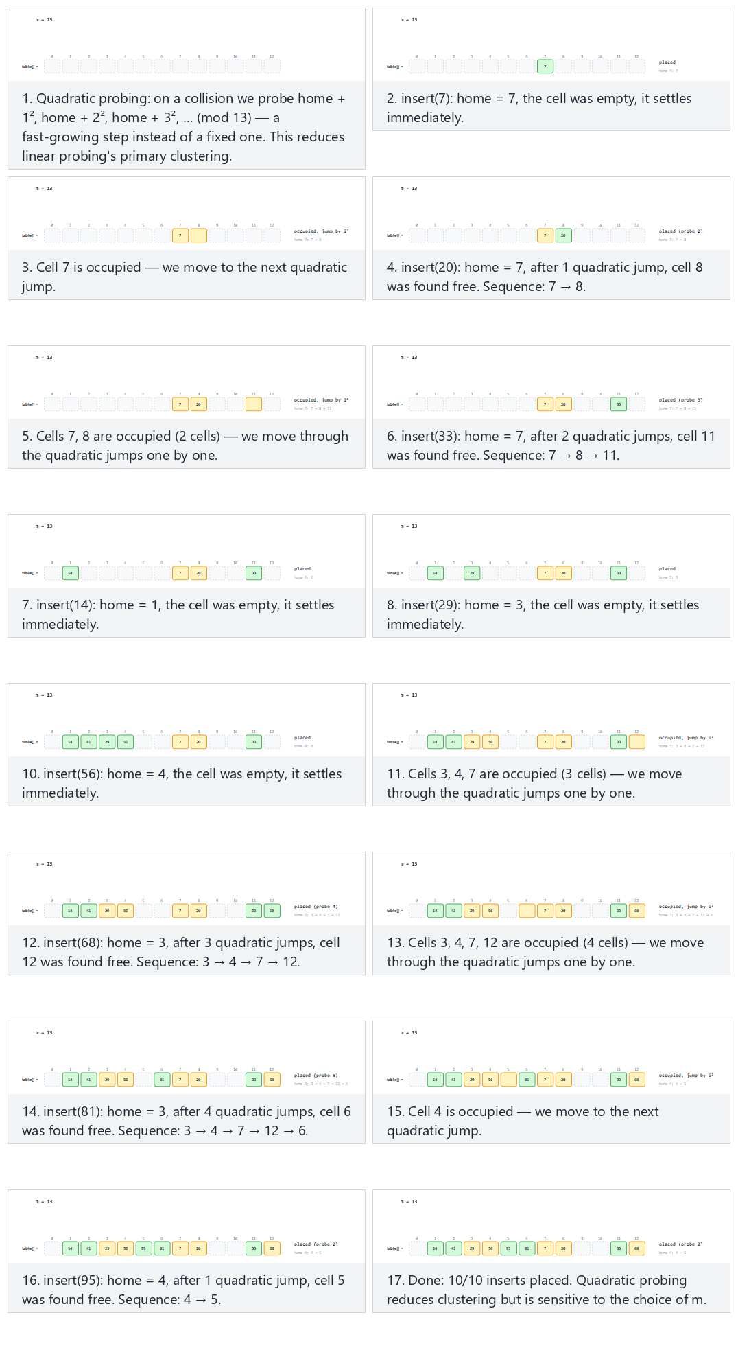
In the picker, also try m = 11, two groups share a home: clear i² patterns (hard) and the edge case m = 8 (a power of 2): the cycle never finds the free slot — or press 🎲 for random data, or type your own m and key list.
9.2.4 Try it
Full program: hash_quadratic_probing.c / HashQuadraticProbing.java
/* Week 6 -- Search and Hashing
 * Open addressing with quadratic probing: on a collision, probe
 * home+1^2, home+2^2, home+3^2, ... (mod m) instead of home+1, home+2,
 * home+3 (linear probing). This avoids primary clustering, but if m is not
 * prime (or the load factor is above 0.5) the i^2 sequence can revisit the
 * same few slots forever and never reach a free one, even though the table
 * is not full.
 * CEN207 Data Structures (formerly CE205)
 */
#include <stdio.h>

#define MAX_M 16
typedef enum { EMPTY, OCCUPIED } Slot;
Slot state[MAX_M];
int table[MAX_M];
int M;

static int h(int key) { return ((key % M) + M) % M; }

int insert(int key, int *probes) {
    int home = h(key);
    for (int i = 0; i < M; i++) {
        int idx = (home + i * i) % M;          /* quadratic probing: i^2 offsets */
        (*probes)++;
        if (state[idx] != OCCUPIED) {
            table[idx] = key;
            state[idx] = OCCUPIED;
            return idx;
        }
    }
    return -1;   /* M probes tried: table full, OR (m not prime / alpha > 0.5) the */
                 /* sequence cycled without ever reaching a free slot           */
}

static int occupied_count(void) { int c = 0; for (int i = 0; i < M; i++) if (state[i] == OCCUPIED) c++; return c; }
static void clear_table(void) { for (int i = 0; i < MAX_M; i++) { state[i] = EMPTY; table[i] = 0; } }

static void run_scenario(const char *label, int m, const int keys[], int n) {
    printf("-- %s --\n", label);
    printf("m = %d\n", m);
    M = m;
    clear_table();
    int placed_count = 0, cycled_count = 0;
    for (int i = 0; i < n; i++) {
        int key = keys[i];
        int probes = 0;
        int idx = insert(key, &probes);
        if (idx != -1) {
            placed_count++;
            printf("  insert(%d): home=%d, placed at %d (%d probe%s)\n", key, h(key), idx, probes, probes == 1 ? "" : "s");
        } else {
            int occ = occupied_count();
            int cycled = occ < m;
            if (cycled) { int free_cells = m - occ; cycled_count++; printf("  insert(%d): home=%d, CYCLED -- %d cell%s still empty but never reached\n", key, h(key), free_cells, free_cells == 1 ? "" : "s"); }
            else printf("  insert(%d): home=%d, table full\n", key, h(key));
        }
    }
    printf("summary: %d/%d inserts placed%s\n\n", placed_count, n,
           cycled_count ? (cycled_count == 1 ? ", 1 cycled despite free space existing" : ", multiple cycled despite free space existing") : "");
}

int main(void) {
    int normal[] = {7, 20, 33, 14, 29, 41, 56, 68, 81, 95};
    int hard[] = {4, 15, 26, 37, 48, 9, 20, 31, 42, 53};
    int cycle[] = {8, 9, 12, 26, 19, 5, 14, 16, 7, 24};

    run_scenario("normal: m = 13 (prime), 10 keys, a few i^2 jumps", 13, normal, 10);
    run_scenario("hard: m = 11, two groups share a home: clear i^2 patterns", 11, hard, 10);
    run_scenario("edge: m = 8 (a power of 2), the cycle never finds the free slot", 8, cycle, 10);

    return 0;
}
/* Week 6 -- Search and Hashing
 * Open addressing with quadratic probing: on a collision, probe
 * home+1^2, home+2^2, home+3^2, ... (mod m) instead of home+1, home+2,
 * home+3 (linear probing). This avoids primary clustering, but if m is not
 * prime (or the load factor is above 0.5) the i^2 sequence can revisit the
 * same few slots forever and never reach a free one, even though the table
 * is not full.
 * CEN207 Data Structures (formerly CE205)
 */
public class HashQuadraticProbing {
    static final int EMPTY = 0, OCCUPIED = 1;
    static final int MAX_M = 16;
    static int[] state = new int[MAX_M];
    static int[] table = new int[MAX_M];
    static int m;

    static int h(int key) { return ((key % m) + m) % m; }

    static int insert(int key, int[] probesOut) {
        int home = h(key);
        for (int i = 0; i < m; i++) {
            int idx = (home + i * i) % m;          // quadratic probing: i^2 offsets
            probesOut[0]++;
            if (state[idx] != OCCUPIED) {
                table[idx] = key;
                state[idx] = OCCUPIED;
                return idx;
            }
        }
        return -1;   // m probes tried: table full, OR (m not prime / alpha > 0.5) the
                     // sequence cycled without ever reaching a free slot
    }

    static int occupiedCount() { int c = 0; for (int i = 0; i < m; i++) if (state[i] == OCCUPIED) c++; return c; }
    static void clearTable() { for (int i = 0; i < MAX_M; i++) { state[i] = EMPTY; table[i] = 0; } }

    static void runScenario(String label, int mm, int[] keys) {
        System.out.println("-- " + label + " --");
        System.out.println("m = " + mm);
        m = mm;
        clearTable();
        int placedCount = 0, cycledCount = 0;
        for (int key : keys) {
            int[] probes = {0};
            int idx = insert(key, probes);
            if (idx != -1) {
                placedCount++;
                System.out.println("  insert(" + key + "): home=" + h(key) + ", placed at " + idx + " (" + probes[0] + " probe" + (probes[0] == 1 ? "" : "s") + ")");
            } else {
                int occ = occupiedCount();
                boolean cycled = occ < m;
                if (cycled) {
                    int freeCells = m - occ;
                    cycledCount++;
                    System.out.println("  insert(" + key + "): home=" + h(key) + ", CYCLED -- " + freeCells + " cell" + (freeCells == 1 ? "" : "s") + " still empty but never reached");
                } else {
                    System.out.println("  insert(" + key + "): home=" + h(key) + ", table full");
                }
            }
        }
        System.out.println("summary: " + placedCount + "/" + keys.length + " inserts placed"
                + (cycledCount > 0 ? (cycledCount == 1 ? ", 1 cycled despite free space existing" : ", multiple cycled despite free space existing") : ""));
        System.out.println();
    }

    public static void main(String[] args) {
        int[] normal = {7, 20, 33, 14, 29, 41, 56, 68, 81, 95};
        int[] hard = {4, 15, 26, 37, 48, 9, 20, 31, 42, 53};
        int[] cycle = {8, 9, 12, 26, 19, 5, 14, 16, 7, 24};

        runScenario("normal: m = 13 (prime), 10 keys, a few i^2 jumps", 13, normal);
        runScenario("hard: m = 11, two groups share a home: clear i^2 patterns", 11, hard);
        runScenario("edge: m = 8 (a power of 2), the cycle never finds the free slot", 8, cycle);
    }
}
Try it
Expected output:
-- normal: m = 13 (prime), 10 keys, a few i^2 jumps --
m = 13
  insert(7): home=7, placed at 7 (1 probe)
  insert(20): home=7, placed at 8 (2 probes)
  insert(33): home=7, placed at 11 (3 probes)
  insert(14): home=1, placed at 1 (1 probe)
  insert(29): home=3, placed at 3 (1 probe)
  insert(41): home=2, placed at 2 (1 probe)
  insert(56): home=4, placed at 4 (1 probe)
  insert(68): home=3, placed at 12 (4 probes)
  insert(81): home=3, placed at 6 (5 probes)
  insert(95): home=4, placed at 5 (2 probes)
summary: 10/10 inserts placed

-- hard: m = 11, two groups share a home: clear i^2 patterns --
m = 11
  insert(4): home=4, placed at 4 (1 probe)
  insert(15): home=4, placed at 5 (2 probes)
  insert(26): home=4, placed at 8 (3 probes)
  insert(37): home=4, placed at 2 (4 probes)
  insert(48): home=4, placed at 9 (5 probes)
  insert(9): home=9, placed at 10 (2 probes)
  insert(20): home=9, placed at 7 (4 probes)
  insert(31): home=9, placed at 3 (5 probes)
  insert(42): home=9, placed at 1 (6 probes)
  insert(53): home=9, CYCLED -- 2 cells still empty but never reached
summary: 9/10 inserts placed, 1 cycled despite free space existing

-- edge: m = 8 (a power of 2), the cycle never finds the free slot --
m = 8
  insert(8): home=0, placed at 0 (1 probe)
  insert(9): home=1, placed at 1 (1 probe)
  insert(12): home=4, placed at 4 (1 probe)
  insert(26): home=2, placed at 2 (1 probe)
  insert(19): home=3, placed at 3 (1 probe)
  insert(5): home=5, placed at 5 (1 probe)
  insert(14): home=6, placed at 6 (1 probe)
  insert(16): home=0, CYCLED -- 1 cell still empty but never reached
  insert(7): home=7, placed at 7 (1 probe)
  insert(24): home=0, table full
summary: 8/10 inserts placed, 1 cycled despite free space existing
9.2.5 Complexity, mistakes, self-check
Complexity. Average case close to O(1 / (1 - alpha)), similar to linear probing, but with less clustering in practice for alpha <= 0.5. Worst case O(m), same as linear probing — plus the possibility of a cycle (probing forever without reaching a free slot, as shown above) if m is not prime or alpha > 0.5, which is a distinct failure mode from "table full".
Common mistakes
- Using a table size
mthat is a power of 2 "for a fast modulo". As the "edge" scenario above shows, this is exactly the condition under which thei^2sequence can cycle through only a handful of slots forever. Quadratic probing specifically needsmprime (and, ideally, kept atalpha <= 0.5) to guarantee it eventually visits every slot. - Confusing a cycle with a full table. Both look like "insert failed after
mprobes" from the outside, but they are different situations: a full table genuinely has no room; a cycled insert fails while free slots still exist elsewhere, purely because ofm's choice. Diagnosing which one occurred (as the code above does, by comparing the occupied count tom) matters for fixing the actual problem. - Computing
i * iwithout checking for overflow on very large tables. For the small tables in this course this never matters, but on a production-sized hash table,ican grow large enough thati * ioverflows a 32-bitintbefore the loop naturally terminates — alongaccumulator avoids this.
Self-check: quadratic probing's blind spot
In the "m = 8" scenario above, inserting 16 (home 0) fails with a CYCLED message even though the table is not full. List the sequence of slots 16's probing actually visits, and explain why it never reaches slot 0's neighbours that happen to still be free at that point.
Answer. 16's home is 16 mod 8 = 0. The probe sequence is (0 + i^2) mod 8 for i = 0, 1, 2, 3, ...: 0, 1, 4, 1, 0, 1, 4, 1, 0, ... (since i^2 mod 8 cycles through only {0, 1, 4} forever once i exceeds a few small values — a consequence of 8 not being prime). Slots 0, 1, and 4 are all already occupied at that point in the scenario, and the sequence never produces any other residue, so it can never reach the still-empty slots (like 7, filled only later by a different key with a different home) — a direct demonstration of why m must be prime for quadratic probing to visit every slot eventually.
9.3 Double hashing
9.3.1 A question to start
Linear probing's flaw is that every colliding key retraces the same +1 path. Quadratic probing's flaw is that every colliding key retraces the same +1, +4, +9, … path — better spread, but still the same path for every key that shares a home slot, and vulnerable to the cycling trap above. What if the probe step itself depended on the key being inserted, so that two different keys colliding at the same home slot would, from then on, follow different paths through the table? That is double hashing — and in practice, it gives the best collision behaviour of the three open-addressing techniques.
9.3.2 The idea: a second hash function picks the step
Double hashing uses two hash functions. h1(key) = key mod m picks the home slot, exactly as before. A second function, h2(key) = r - (key mod r) for a prime r < m, computes a step size that belongs to that key specifically: probe(i) = (h1(key) + i * h2(key)) mod m. Because h2 depends on key, two keys that collide at the same home slot almost always get different steps, and therefore diverge onto different paths after the very first collision — unlike linear or quadratic probing, where the path is fixed regardless of which key is involved. The r - (key mod r) formula guarantees h2(key) is always in [1, r] — never 0 (a step of 0 would reprobe the exact same slot forever, an infinite loop).
9.3.3 In memory, and the code
int h1(int key, int m) { return key % m; }
int h2(int key, int r) { return r - (key % r); }        /* r prime, r < m: h2 in [1..r], never 0 */

bool insert(int key) {
    int idx = h1(key, M), step = h2(key, R);
    for (int i = 0; i < M; i++) {
        if (state[idx] != OCCUPIED) {
            table[idx] = key;
            state[idx] = OCCUPIED;
            return true;
        }
        idx = (idx + step) % M;                          /* every collision uses THIS key's own step */
    }
    return false;
}
static int h1(int key, int m) { return key % m; }
static int h2(int key, int r) { return r - (key % r); } // r prime, r < m: h2 in [1..r], never 0

boolean insert(int key) {
    int idx = h1(key, M), step = h2(key, R);
    for (int i = 0; i < M; i++) {
        if (state[idx] != OCCUPIED) {
            table[idx] = key;
            state[idx] = OCCUPIED;
            return true;
        }
        idx = (idx + step) % M;                          // every collision uses THIS key's own step
    }
    return false;
}
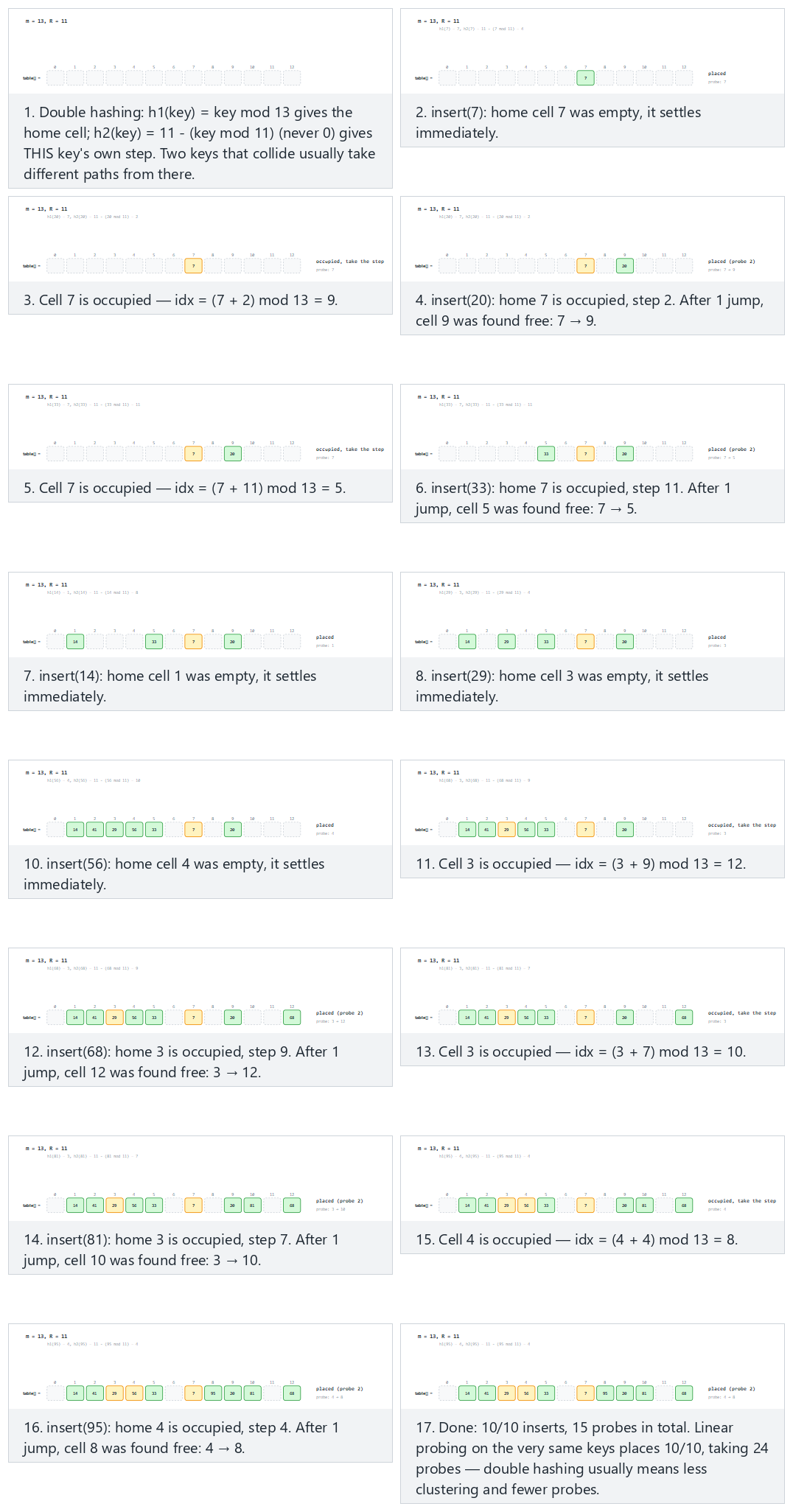
In the picker, also try m = 13, R = 11, many keys share a home (hard) and the edge case m = 9 (not prime): the step shares a factor with m, a cycle forms — or press 🎲 for random data, or type your own m, r, and key list.
9.3.4 Try it
Full program: hash_double_hashing.c / HashDoubleHashing.java
/* Week 6 -- Search and Hashing
 * Open addressing with double hashing: the probe step itself depends on the
 * key, via a second hash function h2. probe(i) = (h1(key) + i * h2(key))
 * mod m. Two keys that collide at the same home cell usually follow
 * different paths from there, unlike linear or quadratic probing where
 * every colliding key retraces the same path.
 * h2(key) = r - (key mod r) for a prime r < m: always in [1..r], so the
 * step is never 0 (a 0 step would reprobe the same cell forever).
 * CEN207 Data Structures (formerly CE205)
 */
#include <stdio.h>

#define MAX_M 16
typedef enum { EMPTY, OCCUPIED } Slot;
Slot state[MAX_M];
int table[MAX_M];
int M, R;

static int h1(int key) { return ((key % M) + M) % M; }
static int h2(int key) { return R - (((key % R) + R) % R); }       /* r prime, r < m: h2 in [1..r], never 0 */

int insert(int key, int *probes) {
    int idx = h1(key), step = h2(key);
    for (int i = 0; i < M; i++) {
        (*probes)++;
        if (state[idx] != OCCUPIED) {
            table[idx] = key;
            state[idx] = OCCUPIED;
            return idx;
        }
        idx = (idx + step) % M;                          /* every collision uses THIS key's own step */
    }
    return -1;
}

/* For the closing comparison ONLY: what linear probing would have done on the same keys.
 * Not used for correctness anywhere -- a separate, simpler simulation. */
static int simulate_linear(const int keys[], int n, int m, int *total_probes) {
    Slot lstate[MAX_M] = {0};
    int placed = 0;
    *total_probes = 0;
    for (int k = 0; k < n; k++) {
        int idx = ((keys[k] % m) + m) % m;
        for (int i = 0; i < m; i++) {
            (*total_probes)++;
            if (!lstate[idx]) { lstate[idx] = OCCUPIED; placed++; break; }
            idx = (idx + 1) % m;
        }
    }
    return placed;
}

static void clear_table(void) { for (int i = 0; i < MAX_M; i++) { state[i] = EMPTY; table[i] = 0; } }
static int occupied_count(void) { int c = 0; for (int i = 0; i < M; i++) if (state[i] == OCCUPIED) c++; return c; }

static void run_scenario(const char *label, int m, int r, const int keys[], int n) {
    printf("-- %s --\n", label);
    printf("m = %d, R = %d\n", m, r);
    M = m; R = r;
    clear_table();
    int placed_count = 0, total_probes = 0, cycled_count = 0;
    for (int i = 0; i < n; i++) {
        int key = keys[i];
        int probes = 0;
        int idx = insert(key, &probes);
        total_probes += probes;
        if (idx != -1) {
            placed_count++;
            printf("  insert(%d): h1=%d h2=%d, placed at %d (%d probe%s)\n",
                   key, h1(key), h2(key), idx, probes, probes == 1 ? "" : "s");
        } else {
            int occ = occupied_count();
            int cycled = occ < m;
            if (cycled) { int free_cells = m - occ; cycled_count++; printf("  insert(%d): h1=%d h2=%d, CYCLED -- %d cell%s still empty but never reached\n", key, h1(key), h2(key), free_cells, free_cells == 1 ? "" : "s"); }
            else printf("  insert(%d): h1=%d h2=%d, table full\n", key, h1(key), h2(key));
        }
    }
    int lin_total = 0;
    int lin_placed = simulate_linear(keys, n, m, &lin_total);
    printf("summary: %d/%d inserts, %d probes in total. Linear probing on the same keys places %d/%d, taking %d probes.\n\n",
           placed_count, n, total_probes, lin_placed, n, lin_total);
    (void) cycled_count;
}

int main(void) {
    int normal[] = {7, 20, 33, 14, 29, 41, 56, 68, 81, 95};
    int hard[] = {4, 17, 30, 43, 56, 8, 21, 34, 47, 60};
    int cycle[] = {13, 16, 10, 9, 2, 3, 5, 6, 4, 17};

    run_scenario("normal: m = 13, R = 11, 10 keys: colliding keys use different steps", 13, 11, normal, 10);
    run_scenario("hard: m = 13, R = 11, many keys share a home", 13, 11, hard, 10);
    run_scenario("edge: m = 9 (not prime), the step shares a factor with m, a cycle forms", 9, 7, cycle, 10);

    return 0;
}
/* Week 6 -- Search and Hashing
 * Open addressing with double hashing: the probe step itself depends on the
 * key, via a second hash function h2. probe(i) = (h1(key) + i * h2(key))
 * mod m. Two keys that collide at the same home cell usually follow
 * different paths from there, unlike linear or quadratic probing where
 * every colliding key retraces the same path.
 * h2(key) = r - (key mod r) for a prime r < m: always in [1..r], so the
 * step is never 0 (a 0 step would reprobe the same cell forever).
 * CEN207 Data Structures (formerly CE205)
 */
public class HashDoubleHashing {
    static final int EMPTY = 0, OCCUPIED = 1;
    static final int MAX_M = 16;
    static int[] state = new int[MAX_M];
    static int[] table = new int[MAX_M];
    static int m, r;

    static int h1(int key) { return ((key % m) + m) % m; }
    static int h2(int key) { return r - (((key % r) + r) % r); } // r prime, r < m: h2 in [1..r], never 0

    static int insert(int key, int[] probesOut) {
        int idx = h1(key), step = h2(key);
        for (int i = 0; i < m; i++) {
            probesOut[0]++;
            if (state[idx] != OCCUPIED) {
                table[idx] = key;
                state[idx] = OCCUPIED;
                return idx;
            }
            idx = (idx + step) % m;                          // every collision uses THIS key's own step
        }
        return -1;
    }

    /* For the closing comparison ONLY: what linear probing would have done on the same keys.
     * Not used for correctness anywhere -- a separate, simpler simulation. */
    static int simulateLinear(int[] keys, int mm, int[] totalOut) {
        boolean[] lstate = new boolean[MAX_M];
        int placed = 0;
        totalOut[0] = 0;
        for (int key : keys) {
            int idx = ((key % mm) + mm) % mm;
            for (int i = 0; i < mm; i++) {
                totalOut[0]++;
                if (!lstate[idx]) { lstate[idx] = true; placed++; break; }
                idx = (idx + 1) % mm;
            }
        }
        return placed;
    }

    static void clearTable() { for (int i = 0; i < MAX_M; i++) { state[i] = EMPTY; table[i] = 0; } }
    static int occupiedCount() { int c = 0; for (int i = 0; i < m; i++) if (state[i] == OCCUPIED) c++; return c; }

    static void runScenario(String label, int mm, int rr, int[] keys) {
        System.out.println("-- " + label + " --");
        System.out.println("m = " + mm + ", R = " + rr);
        m = mm; r = rr;
        clearTable();
        int placedCount = 0, totalProbes = 0;
        for (int key : keys) {
            int[] probes = {0};
            int idx = insert(key, probes);
            totalProbes += probes[0];
            if (idx != -1) {
                placedCount++;
                System.out.println("  insert(" + key + "): h1=" + h1(key) + " h2=" + h2(key) + ", placed at " + idx + " (" + probes[0] + " probe" + (probes[0] == 1 ? "" : "s") + ")");
            } else {
                int occ = occupiedCount();
                boolean cycled = occ < m;
                if (cycled) {
                    int freeCells = m - occ;
                    System.out.println("  insert(" + key + "): h1=" + h1(key) + " h2=" + h2(key) + ", CYCLED -- " + freeCells + " cell" + (freeCells == 1 ? "" : "s") + " still empty but never reached");
                } else {
                    System.out.println("  insert(" + key + "): h1=" + h1(key) + " h2=" + h2(key) + ", table full");
                }
            }
        }
        int[] linTotal = {0};
        int linPlaced = simulateLinear(keys, m, linTotal);
        System.out.println("summary: " + placedCount + "/" + keys.length + " inserts, " + totalProbes + " probes in total. Linear probing on the same keys places "
                + linPlaced + "/" + keys.length + ", taking " + linTotal[0] + " probes.");
        System.out.println();
    }

    public static void main(String[] args) {
        int[] normal = {7, 20, 33, 14, 29, 41, 56, 68, 81, 95};
        int[] hard = {4, 17, 30, 43, 56, 8, 21, 34, 47, 60};
        int[] cycle = {13, 16, 10, 9, 2, 3, 5, 6, 4, 17};

        runScenario("normal: m = 13, R = 11, 10 keys: colliding keys use different steps", 13, 11, normal);
        runScenario("hard: m = 13, R = 11, many keys share a home", 13, 11, hard);
        runScenario("edge: m = 9 (not prime), the step shares a factor with m, a cycle forms", 9, 7, cycle);
    }
}
Try it
Expected output:
-- normal: m = 13, R = 11, 10 keys: colliding keys use different steps --
m = 13, R = 11
  insert(7): h1=7 h2=4, placed at 7 (1 probe)
  insert(20): h1=7 h2=2, placed at 9 (2 probes)
  insert(33): h1=7 h2=11, placed at 5 (2 probes)
  insert(14): h1=1 h2=8, placed at 1 (1 probe)
  insert(29): h1=3 h2=4, placed at 3 (1 probe)
  insert(41): h1=2 h2=3, placed at 2 (1 probe)
  insert(56): h1=4 h2=10, placed at 4 (1 probe)
  insert(68): h1=3 h2=9, placed at 12 (2 probes)
  insert(81): h1=3 h2=7, placed at 10 (2 probes)
  insert(95): h1=4 h2=4, placed at 8 (2 probes)
summary: 10/10 inserts, 15 probes in total. Linear probing on the same keys places 10/10, taking 24 probes.

-- hard: m = 13, R = 11, many keys share a home --
m = 13, R = 11
  insert(4): h1=4 h2=7, placed at 4 (1 probe)
  insert(17): h1=4 h2=5, placed at 9 (2 probes)
  insert(30): h1=4 h2=3, placed at 7 (2 probes)
  insert(43): h1=4 h2=1, placed at 5 (2 probes)
  insert(56): h1=4 h2=10, placed at 1 (2 probes)
  insert(8): h1=8 h2=3, placed at 8 (1 probe)
  insert(21): h1=8 h2=1, placed at 10 (3 probes)
  insert(34): h1=8 h2=10, placed at 2 (3 probes)
  insert(47): h1=8 h2=8, placed at 3 (2 probes)
  insert(60): h1=8 h2=6, placed at 0 (4 probes)
summary: 10/10 inserts, 22 probes in total. Linear probing on the same keys places 10/10, taking 35 probes.

-- edge: m = 9 (not prime), the step shares a factor with m, a cycle forms --
m = 9, R = 7
  insert(13): h1=4 h2=1, placed at 4 (1 probe)
  insert(16): h1=7 h2=5, placed at 7 (1 probe)
  insert(10): h1=1 h2=4, placed at 1 (1 probe)
  insert(9): h1=0 h2=5, placed at 0 (1 probe)
  insert(2): h1=2 h2=5, placed at 2 (1 probe)
  insert(3): h1=3 h2=4, placed at 3 (1 probe)
  insert(5): h1=5 h2=2, placed at 5 (1 probe)
  insert(6): h1=6 h2=1, placed at 6 (1 probe)
  insert(4): h1=4 h2=3, CYCLED -- 1 cell still empty but never reached
  insert(17): h1=8 h2=4, placed at 8 (1 probe)
summary: 9/10 inserts, 18 probes in total. Linear probing on the same keys places 9/10, taking 22 probes.
9.3.5 Complexity, mistakes, self-check
Complexity. Average case close to O(1 / (1 - alpha)), with the least clustering of the three open-addressing techniques in practice — the "normal" scenario above needed 15 probes in total versus linear probing's 24 on the exact same keys. Worst case still O(m), and still vulnerable to cycling if step (h2(key)) shares a common factor with m — exactly why m should be prime here too, and r a smaller prime.
Common mistakes
- Letting
h2(key)possibly return 0. A step of0means "probe the same slot forever" — an infinite loop that never terminates, since it can never move away from an occupied slot. Ther - (key mod r)formula is specifically designed to always land in[1, r], guaranteeing a non-zero step. - Choosing
rnot prime, orr >= m. The formula's guarantee (step is always a "good" divisor-free value relative tom) depends onrbeing a prime smaller thanm— an arbitraryrreintroduces the same clustering risk double hashing exists to avoid. - Assuming double hashing can never cycle. As the "edge" scenario shows (
m = 9, not prime), it still can, for the same underlying reason as quadratic probing: if the step andmshare a common factor, the probe sequence only ever visits a subset of the table's slots.
Self-check: why double hashing usually beats linear probing
In the "hard: m = 13, R = 11, many keys share a home" scenario, five keys (4, 17, 30, 43, 56) all hash to the same home slot, 4. Explain why double hashing still places all of them with only 2–3 probes each (never retracing another colliding key's exact path), while linear probing on the same keys would have to place them in five consecutive slots, 4, 5, 6, 7, 8, growing one long cluster.
Answer. Each of those five keys has a different h2 value (7, 5, 3, 1, 10 respectively, computed from 11 - (key mod 11)), so once two of them collide, they immediately diverge onto different step sizes — 4's step is 7, 17's is 5, and so on — landing in different, often non-adjacent slots rather than all queuing up one after another. Linear probing, by contrast, always uses the fixed step 1 for every key regardless of which key it is, so all five would necessarily occupy one unbroken run of consecutive slots — exactly the primary-clustering behaviour double hashing is designed to avoid.
10. Rehashing and amortized cost
10.1 A question to start
Every open-addressing technique above has a hard wall: once the load factor alpha = n/m gets close to 1 (linear probing) or 0.5 (quadratic probing), performance degrades sharply, and eventually — once m slots are genuinely occupied — insertion simply fails, no matter which probing rule you use. Even separate chaining, which never technically "fails", degrades toward O(n) search as alpha grows without bound. A hash table cannot know in advance how many keys it will eventually hold, so it needs a way to grow itself once it starts filling up. That is rehashing.
10.2 The idea: grow, and move every key
When the load factor crosses a chosen threshold (a common choice is 0.8), the table allocates a new, larger array — conventionally the next prime number at least double the current size — and reinserts every key currently in the table into the new one, from scratch. This last part is essential and easy to miss: because the table size m changed, h(key) = key mod m computes a different index for most keys in the new table than it did in the old one, so simply copying the old array over would place most keys in the wrong slot. Every key must be recomputed and reinserted individually.
10.3 Amortized cost: why rehashing does not ruin O(1) insertion
A single rehash is expensive: it touches every key currently in the table, an O(n) operation. Does this mean insertion is not really O(1) after all? The answer is amortized analysis: rehashing happens rarely — by doubling the table size each time, the next rehash cannot happen again until roughly n more insertions have occurred (the table has to fill back up to the threshold first) — so the total cost of all the rehashes across a long sequence of n insertions, spread evenly across those n insertions, works out to a small constant amount of extra work per insertion. This "doubling keeps the average cheap even though individual operations are occasionally expensive" pattern is the same idea behind a dynamic array's realloc-and-copy growth strategy, if you have seen that in another course — rehashing is the hash-table version of exactly that trick.
10.4 In memory, and the code
double threshold = 0.8;
Slot *state; int *table; int m, n;    /* current table, its size, and how many keys are in it */

int is_prime(int x) {
    if (x < 2) return 0;
    for (int i = 2; (long) i * i <= x; i++) if (x % i == 0) return 0;
    return 1;
}
int next_prime(int x) { while (!is_prime(x)) x++; return x; }

int insert_into(Slot *st, int *tb, int mm, int key) {         /* returns the index used */
    int idx = key % mm;
    for (int i = 0; i < mm; i++) {
        if (st[idx] != OCCUPIED) { tb[idx] = key; st[idx] = OCCUPIED; return idx; }
        idx = (idx + 1) % mm;
    }
    return -1;
}

void rehash(void) {
    int newM = next_prime(2 * m);
    Slot *newState = calloc(newM, sizeof(Slot));
    int *newTable = malloc(newM * sizeof(int));
    for (int i = 0; i < m; i++)
        if (state[i] == OCCUPIED) insert_into(newState, newTable, newM, table[i]);   /* every key moves */
    free(state); free(table);
    state = newState; table = newTable; m = newM;
}

void insert(int key) {
    insert_into(state, table, m, key);
    n++;
    if ((double) n / m > threshold) rehash();
}
static final double THRESHOLD = 0.8;
int[] state; int[] table; int m, n;   // current table, its size, and how many keys are in it

static boolean isPrime(int x) {
    if (x < 2) return false;
    for (int i = 2; (long) i * i <= x; i++) if (x % i == 0) return false;
    return true;
}
static int nextPrime(int x) { while (!isPrime(x)) x++; return x; }

int insertInto(int[] st, int[] tb, int mm, int key) {         // returns the index used
    int idx = key % mm;
    for (int i = 0; i < mm; i++) {
        if (st[idx] != OCCUPIED) { tb[idx] = key; st[idx] = OCCUPIED; return idx; }
        idx = (idx + 1) % mm;
    }
    return -1;
}

void rehash() {
    int newM = nextPrime(2 * m);
    int[] newState = new int[newM], newTable = new int[newM];
    for (int i = 0; i < m; i++)
        if (state[i] == OCCUPIED) insertInto(newState, newTable, newM, table[i]);   // every key moves
    state = newState; table = newTable; m = newM;
}

void insert(int key) {
    insertInto(state, table, m, key);
    n++;
    if ((double) n / m > THRESHOLD) rehash();
}
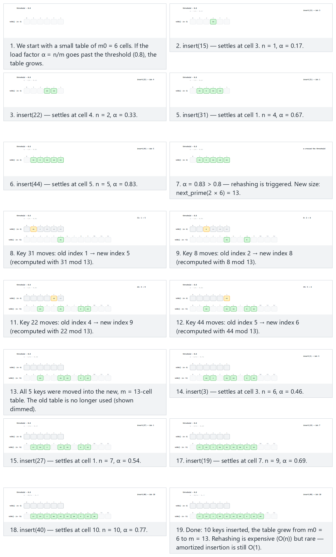
In the picker, also try m0 = 6, keys cluster at the same home, growing relieves it (hard) and the edge case m0 = 2: a tiny table grows twice in a row — or press 🎲 for random data, or type your own starting size, threshold, and key list.
10.5 Try it
Full program: rehashing.c / Rehashing.java
/* Week 6 -- Search and Hashing
 * Rehashing: open addressing (linear probing) works only while the table
 * has room. When the load factor n/m goes past a threshold, we allocate a
 * bigger table -- size = the next prime at least 2*m -- and reinsert every
 * key into it from scratch (every key's index can change, since the
 * modulus changed). This keeps the average probe length bounded as the
 * table grows.
 * CEN207 Data Structures (formerly CE205)
 */
#include <stdio.h>
#include <stdlib.h>

typedef enum { EMPTY, OCCUPIED } Slot;
double threshold = 0.8;
Slot *state; int *table; int m, n;    /* current table, its size, and how many keys are in it */

int is_prime(int x) {
    if (x < 2) return 0;
    for (int i = 2; (long) i * i <= x; i++) if (x % i == 0) return 0;
    return 1;
}
int next_prime(int x) { while (!is_prime(x)) x++; return x; }

int insert_into(Slot *st, int *tb, int mm, int key) {         /* returns the index used */
    int idx = ((key % mm) + mm) % mm;
    for (int i = 0; i < mm; i++) {
        if (st[idx] != OCCUPIED) { tb[idx] = key; st[idx] = OCCUPIED; return idx; }
        idx = (idx + 1) % mm;
    }
    return -1;
}

void rehash(void) {
    int new_m = next_prime(2 * m);
    Slot *new_state = calloc(new_m, sizeof(Slot));
    int *new_table = malloc(new_m * sizeof(int));
    printf("  rehash: alpha exceeded %.2f, growing table %d -> %d\n", threshold, m, new_m);
    for (int i = 0; i < m; i++) {
        if (state[i] == OCCUPIED) {
            int new_idx = insert_into(new_state, new_table, new_m, table[i]);
            printf("    move key %d: old index %d -> new index %d\n", table[i], i, new_idx);
        }
    }
    free(state); free(table);
    state = new_state; table = new_table; m = new_m;
}

void insert(int key) {
    int idx = insert_into(state, table, m, key);
    n++;
    printf("  insert(%d): placed at %d, n=%d, m=%d, alpha=%.2f\n", key, idx, n, m, (double) n / m);
    if ((double) n / m > threshold) rehash();
}

static void run_scenario(const char *label, int m0, double thr, const int keys[], int count) {
    printf("-- %s --\n", label);
    printf("m0 = %d, threshold = %.2f\n", m0, thr);
    threshold = thr;
    m = m0; n = 0;
    state = calloc(m, sizeof(Slot));
    table = malloc(m * sizeof(int));
    for (int i = 0; i < count; i++) insert(keys[i]);
    printf("summary: %d keys inserted, table grew from %d to %d, final alpha=%.2f\n\n", n, m0, m, (double) n / m);
    free(state); free(table);
}

int main(void) {
    int normal[] = {15, 22, 8, 31, 44, 3, 27, 56, 19, 40};
    int hard[] = {12, 18, 24, 30, 36, 7, 13, 19, 25, 31};
    int double_rehash[] = {5, 12, 19, 26, 9, 16};

    run_scenario("normal: m0 = 6, 10 keys: grows once", 6, 0.8, normal, 10);
    run_scenario("hard: m0 = 6, keys cluster at the same home, growing relieves it", 6, 0.8, hard, 10);
    run_scenario("edge: m0 = 2, a tiny table grows twice in a row", 2, 0.8, double_rehash, 6);

    return 0;
}
/* Week 6 -- Search and Hashing
 * Rehashing: open addressing (linear probing) works only while the table
 * has room. When the load factor n/m goes past a threshold, we allocate a
 * bigger table -- size = the next prime at least 2*m -- and reinsert every
 * key into it from scratch (every key's index can change, since the
 * modulus changed). This keeps the average probe length bounded as the
 * table grows.
 * CEN207 Data Structures (formerly CE205)
 */
public class Rehashing {
    static final int EMPTY = 0, OCCUPIED = 1;
    static double threshold = 0.8;
    static int[] state; static int[] table; static int m, n;   // current table, its size, and how many keys are in it

    static boolean isPrime(int x) {
        if (x < 2) return false;
        for (int i = 2; (long) i * i <= x; i++) if (x % i == 0) return false;
        return true;
    }
    static int nextPrime(int x) { while (!isPrime(x)) x++; return x; }

    static int insertInto(int[] st, int[] tb, int mm, int key) {         // returns the index used
        int idx = ((key % mm) + mm) % mm;
        for (int i = 0; i < mm; i++) {
            if (st[idx] != OCCUPIED) { tb[idx] = key; st[idx] = OCCUPIED; return idx; }
            idx = (idx + 1) % mm;
        }
        return -1;
    }

    static void rehash() {
        int newM = nextPrime(2 * m);
        int[] newState = new int[newM], newTable = new int[newM];
        System.out.println("  rehash: alpha exceeded " + String.format("%.2f", threshold) + ", growing table " + m + " -> " + newM);
        for (int i = 0; i < m; i++) {
            if (state[i] == OCCUPIED) {
                int newIdx = insertInto(newState, newTable, newM, table[i]);
                System.out.println("    move key " + table[i] + ": old index " + i + " -> new index " + newIdx);
            }
        }
        state = newState; table = newTable; m = newM;
    }

    static void insert(int key) {
        int idx = insertInto(state, table, m, key);
        n++;
        System.out.println("  insert(" + key + "): placed at " + idx + ", n=" + n + ", m=" + m + ", alpha=" + String.format("%.2f", (double) n / m));
        if ((double) n / m > threshold) rehash();
    }

    static void runScenario(String label, int m0, double thr, int[] keys) {
        System.out.println("-- " + label + " --");
        System.out.println("m0 = " + m0 + ", threshold = " + String.format("%.2f", thr));
        threshold = thr;
        m = m0; n = 0;
        state = new int[m];
        table = new int[m];
        for (int key : keys) insert(key);
        System.out.println("summary: " + n + " keys inserted, table grew from " + m0 + " to " + m + ", final alpha=" + String.format("%.2f", (double) n / m));
        System.out.println();
    }

    public static void main(String[] args) {
        int[] normal = {15, 22, 8, 31, 44, 3, 27, 56, 19, 40};
        int[] hard = {12, 18, 24, 30, 36, 7, 13, 19, 25, 31};
        int[] doubleRehash = {5, 12, 19, 26, 9, 16};

        runScenario("normal: m0 = 6, 10 keys: grows once", 6, 0.8, normal);
        runScenario("hard: m0 = 6, keys cluster at the same home, growing relieves it", 6, 0.8, hard);
        runScenario("edge: m0 = 2, a tiny table grows twice in a row", 2, 0.8, doubleRehash);
    }
}
Try it
Expected output:
-- normal: m0 = 6, 10 keys: grows once --
m0 = 6, threshold = 0.80
  insert(15): placed at 3, n=1, m=6, alpha=0.17
  insert(22): placed at 4, n=2, m=6, alpha=0.33
  insert(8): placed at 2, n=3, m=6, alpha=0.50
  insert(31): placed at 1, n=4, m=6, alpha=0.67
  insert(44): placed at 5, n=5, m=6, alpha=0.83
  rehash: alpha exceeded 0.80, growing table 6 -> 13
    move key 31: old index 1 -> new index 5
    move key 8: old index 2 -> new index 8
    move key 15: old index 3 -> new index 2
    move key 22: old index 4 -> new index 9
    move key 44: old index 5 -> new index 6
  insert(3): placed at 3, n=6, m=13, alpha=0.46
  insert(27): placed at 1, n=7, m=13, alpha=0.54
  insert(56): placed at 4, n=8, m=13, alpha=0.62
  insert(19): placed at 7, n=9, m=13, alpha=0.69
  insert(40): placed at 10, n=10, m=13, alpha=0.77
summary: 10 keys inserted, table grew from 6 to 13, final alpha=0.77

-- hard: m0 = 6, keys cluster at the same home, growing relieves it --
m0 = 6, threshold = 0.80
  insert(12): placed at 0, n=1, m=6, alpha=0.17
  insert(18): placed at 1, n=2, m=6, alpha=0.33
  insert(24): placed at 2, n=3, m=6, alpha=0.50
  insert(30): placed at 3, n=4, m=6, alpha=0.67
  insert(36): placed at 4, n=5, m=6, alpha=0.83
  rehash: alpha exceeded 0.80, growing table 6 -> 13
    move key 12: old index 0 -> new index 12
    move key 18: old index 1 -> new index 5
    move key 24: old index 2 -> new index 11
    move key 30: old index 3 -> new index 4
    move key 36: old index 4 -> new index 10
  insert(7): placed at 7, n=6, m=13, alpha=0.46
  insert(13): placed at 0, n=7, m=13, alpha=0.54
  insert(19): placed at 6, n=8, m=13, alpha=0.62
  insert(25): placed at 1, n=9, m=13, alpha=0.69
  insert(31): placed at 8, n=10, m=13, alpha=0.77
summary: 10 keys inserted, table grew from 6 to 13, final alpha=0.77

-- edge: m0 = 2, a tiny table grows twice in a row --
m0 = 2, threshold = 0.80
  insert(5): placed at 1, n=1, m=2, alpha=0.50
  insert(12): placed at 0, n=2, m=2, alpha=1.00
  rehash: alpha exceeded 0.80, growing table 2 -> 5
    move key 12: old index 0 -> new index 2
    move key 5: old index 1 -> new index 0
  insert(19): placed at 4, n=3, m=5, alpha=0.60
  insert(26): placed at 1, n=4, m=5, alpha=0.80
  insert(9): placed at 3, n=5, m=5, alpha=1.00
  rehash: alpha exceeded 0.80, growing table 5 -> 11
    move key 5: old index 0 -> new index 5
    move key 26: old index 1 -> new index 4
    move key 12: old index 2 -> new index 1
    move key 9: old index 3 -> new index 9
    move key 19: old index 4 -> new index 8
  insert(16): placed at 6, n=6, m=11, alpha=0.55
summary: 6 keys inserted, table grew from 2 to 11, final alpha=0.55
10.6 Complexity, mistakes, self-check
Complexity. A single rehash: O(n) — every occupied slot is revisited and reinserted. Amortized over a long sequence of insertions with table doubling: O(1) amortized per insertion — the same guarantee dynamic arrays give you for push/append, applied to a hash table's grow operation. The rehash threshold itself is a tuning knob: a lower threshold rehashes more often (more overhead) but keeps alpha — and therefore per-operation cost — lower at all times; a higher threshold rehashes less often but lets alpha, and per-operation cost, climb higher between rehashes.
Common mistakes
- Growing the table by a fixed increment (
m + 10) instead of doubling (2 * m, rounded up to the next prime). Fixed-increment growth means the table must rehash every10insertions forever, making the total rehashing cost acrossninsertionsO(n^2 / 10)instead ofO(n)— the amortizedO(1)guarantee is lost entirely. - Forgetting that every key's index can change after a rehash. Any code elsewhere that cached an index returned by an earlier
insertcall (rather than always recomputingh(key)against the currentm) will silently break the moment a rehash happens — this is exactly why hash tables you use from a standard library (Java'sHashMap, for instance) never expose raw indices to you at all. - Checking the load factor before inserting instead of after. The threshold check must happen after the new key is placed and
nincremented (as the code above does), so that the table always rehashes in response to what it actually holds, not what it is about to hold.
Self-check: why does the table grow to a prime, not just double?
In the "normal" scenario above, m0 = 6 grows to 13 (not 12) after the first rehash. Why does next_prime(2 * m) matter here, given everything you learned about m in sections 7 and 9?
Answer. Doubling alone (6 -> 12) would hand the new table exactly the same "m is not prime" vulnerability that sections 7.4 and 9.2.2 warned about — a table size with small common factors clusters keys badly under the division method, and can even cause quadratic or double hashing to cycle (section 9.2/9.3). Rounding the doubled size up to the next prime (12 -> 13) keeps the new, larger table just as resistant to clustering as a carefully chosen initial m would have been.
11. Choosing a technique
| Situation | Best choice | Why |
|---|---|---|
| Data is sorted, and you just need occasional lookups, no insert/delete | Binary search (Week 1) | Simplest correct O(log n) tool; no extra memory |
| Sorted, need to minimize division operations (rare, constrained hardware) | Fibonacci search | Same O(log n), addition/subtraction only |
| Sorted, memory access pattern matters more than comparison count | Jump search | Sequential block scan, simple arithmetic, O(sqrt n) |
| Sorted, numeric, known to be roughly uniformly distributed | Interpolation search | O(log log n) average — the fastest comparison-based option here |
Sorted, target is very likely near the front, or n is unknown/huge | Exponential search | Cost scales with the target's actual position, not n |
| Frequent insert/search/delete by key, order does not matter, deletions are common | Hashing with separate chaining | Simple deletion (no tombstones needed), degrades gracefully |
| Frequent insert/search by key, memory locality matters, deletions are rare | Hashing with open addressing (double hashing preferred) | No linked-list overhead, best cache behaviour, avoids most clustering |
| Any hash table whose key count will grow substantially over its lifetime | Hashing + rehashing | Keeps alpha bounded, preserving O(1) amortized cost as n grows |
The single biggest decision is not actually "which search technique" — it is "do I need the data sorted for some other reason (range queries, in-order iteration, finding the minimum/maximum quickly), or do I only ever need exact-match lookups?" If only exact-match lookups matter, a well-configured hash table almost always wins over any of the four comparison-based techniques from sections 2–5, because O(1) average case beats even O(log log n). Sorted-order techniques remain essential exactly when you need more than lookup — which is why this course keeps teaching both families side by side.
Summary
This week added four new comparison-based searches to the linear and binary search you already knew — jump search (fixed blocks, O(sqrt n)), interpolation search (a formula estimate, O(log log n) on uniform data but O(n) worst case), exponential search (double a bound, then binary search, cost scales with the target's actual position), and Fibonacci search (Fibonacci-number splits, O(log n) using only addition and subtraction) — and then introduced a genuinely different idea: the hash table, which computes a key's location directly with a hash function (the division method, h(k) = k mod m, with m chosen prime) instead of comparing and narrowing. Because two keys can hash to the same slot, every hash table needs a collision resolution strategy: separate chaining (a linked list per slot, simple, degrades gracefully) or open addressing (every key lives inside the table itself — linear probing, simple but prone to primary clustering; quadratic probing, spreads better but needs m prime and alpha <= 0.5; double hashing, the best practical spread, using a second, key-dependent step). Finally, rehashing — doubling the table and moving every key when the load factor crosses a threshold — keeps a hash table's O(1) average-case performance intact as it grows, at an amortized O(1) cost per insertion despite each individual rehash costing O(n).
Exercises
- Derive, from first principles (not by looking it up), why jump search's optimal block size is
b = sqrt(n), by minimizingf(b) = n/b + b. State the resulting worst-case comparison count in terms ofn. - Modify
interpolation_search.cso that, alongside its existing guard forarr[hi] == arr[lo], it also prints a warning the first time the estimatedposfalls more thann/2away from the range's true midpoint(lo + hi) / 2— a rough signal that the data may be skewed. Test it against the "skewed" scenario from section 3. - Trace
exponential_search.c's bound-finding phase by hand for an array ofn = 1000elements, assuming the target is at index130. How many bound-finding comparisons does it take, and what is the resulting[lo, hi]range handed to the binary-search phase? - In
fibonacci_search.c, the Fibonacci triple shrinks by one step when eliminating the left part and by two steps when eliminating the right part. Trace by hand what would go wrong (which index would be computed incorrectly) if this were reversed — left eliminating by two steps and right by one. - Using
hash_division.c'shash_divisionfunction, find a set of 5 distinct keys and a value ofm(not necessarily prime) that produces zero collisions, and a second set of 5 distinct keys that produces the maximum possible number of collisions (all 5 landing in one slot) for the samem. - Modify
hash_chaining.cto add adelete_keyfunction (search the target key's chain and unlink its node). Unlike open addressing'sdelete_key, explain in one sentence why separate chaining's deletion needs no tombstone at all. - Using
hash_linear_probing.c's "table-full" scenario (m = 8, 8 keys all colliding into slot 3), compute by hand whatalpha(load factor) would be immediately before a rehash triggered at threshold0.8, versus this scenario's actual finalalphaof1.0(no rehashing implemented in that file). Explain in one sentence why this specific scenario is a worst case for linear probing regardless ofm's primality. hash_quadratic_probing.c's "edge" scenario (m = 8) shows a key cycling despite free slots existing. Pick a different, larger power of 2 (saym = 16) and a set of 10 keys that would reproduce the same kind of cycling failure; explain your reasoning.- Using
hash_double_hashing.c'ssimulate_linearfunction as a model, write (in words, no need to implement it) asimulate_quadraticfunction that would let you compare double hashing's total probe count against quadratic probing's, on the same key set. What would you expect the comparison to show, and why? - Trace
rehashing.c'srehashfunction by hand for a table withm = 5, currently holding keys{3, 8, 13, 18}at indices{3, 8 mod 5 = 3 -> probed to 4, 13 mod 5 = 3 -> probed to 0, 18 mod 5 = 3 -> probed to 1}(i.e., all four collided at home slot 3 and probed forward). After rehashing tonext_prime(10) = 11, which new index does each key land at, and does any of them still collide with another?
Self-check quiz
1. Why is jump search's O(sqrt(n)) worse than binary search's O(log n), and what does jump search gain in exchange?
For any n larger than a handful of elements, sqrt(n) grows much faster than log2(n) (for n = 1,000,000, sqrt(n) = 1000 versus log2(n) ≈ 20), so jump search needs far more comparisons in the worst case. In exchange, it needs only addition (no division/shift arithmetic for a midpoint) and accesses memory in short sequential runs within each block, rather than jumping unpredictably across the whole array the way binary search does.
2. Why can interpolation search's worst case be O(n), even though its average case on uniform data is O(log log n)?
The formula's accuracy depends entirely on the assumption that values are roughly evenly spread between arr[lo] and arr[hi]. On skewed data — a cluster of close values plus one far outlier, for instance — the formula's estimate is pulled badly off target, and each probe eliminates only a tiny sliver of the range instead of roughly half, degrading toward the same cost as a linear scan.
3. In exponential search, why is the bound-finding phase's cost O(log index) rather than O(log n)?
The bound doubles — 1, 2, 4, 8, ... — only until it first reaches or passes the target's actual position (index), not until it reaches n. The number of doublings needed to exceed index is log2(index), which can be far smaller than log2(n) when the target is near the front of a very large array.
4. What historical constraint motivated Fibonacci search's "no division or multiplication" design, and how does maintaining the Fibonacci triple (fib, fib1, fib2) achieve it?
On early computing hardware, and still on some constrained embedded processors, division is substantially more expensive than addition or subtraction. Because Fibonacci numbers satisfy fib = fib1 + fib2 exactly, the three running values can be updated at every step using only addition and subtraction, without ever needing to divide the range to find a probe position.
5. What historical idea is hashing's "compute the location, don't search for it" principle credited to, and how does it differ fundamentally from every search technique in sections 2–5?
It is credited to Hans Peter Luhn's 1953 internal IBM memorandum proposing direct-computed table addresses instead of stored or searched order. Every technique in sections 2–5 is still fundamentally comparison-based — it narrows a range by comparing target against stored values. Hashing abandons comparison-and-narrowing entirely: the hash function computes the answer's location directly from the key, in O(1), independent of how many other keys are already stored.
6. Why must a table size m chosen for the division hash method usually be prime, and what specifically goes wrong when it shares a factor with the key pattern?
If m and the keys (or the differences between keys) share a common factor d, every one of those keys hashes to a multiple of d within [0, m) — a small subset of the available slots — causing heavy clustering regardless of how many distinct keys there are. A prime m, having no small factors in common with typical key patterns, spreads keys far more evenly for most real data (though it is a heuristic, not an absolute guarantee, as section 7's "hard" scenario showed).
7. In separate chaining, why is search's average cost expressed as O(1 + alpha) rather than simply O(alpha)?
The 1 accounts for the O(1) cost of computing the hash function itself and locating the correct bucket — a fixed cost paid on every search regardless of chain length. The alpha (the load factor, n/m) is the additional average cost of walking the chain once you have found the right bucket. Both parts matter: even with an empty chain (alpha near 0), a search still costs the constant hashing overhead.
8. What is primary clustering in linear probing, and why does quadratic probing reduce it while introducing a different problem instead?
Primary clustering is the snowball effect where an occupied run of consecutive slots grows because it is more likely to catch the next colliding key too, which then makes the run even longer. Quadratic probing's fast-growing i^2 step spreads colliding keys out much faster, avoiding that specific snowball — but its fixed probe sequence (the same i^2 pattern for every key, regardless of which key it is) can cycle through only a small subset of the table's slots forever if m is not prime or alpha > 0.5, even when free slots genuinely exist elsewhere.
9. Why does double hashing typically outperform both linear and quadratic probing in practice, in one sentence?
Because the probe step itself (h2(key)) depends on the key being inserted, two keys that collide at the same home slot almost always diverge onto different paths immediately, rather than every colliding key retracing the exact same fixed sequence of offsets the way linear probing (+1, +1, ...) and quadratic probing (+1, +4, +9, ...) both do.
10. Why is rehashing's O(n) cost per individual rehash compatible with claiming O(1) amortized insertion cost overall?
Because the table size doubles at each rehash, the number of insertions that must occur before the next rehash is triggered grows in proportion to the table's new size — so, spread evenly across all the insertions that happen between one rehash and the next, the total rehashing work across any long sequence of n insertions works out to a small constant amount of extra work per insertion, exactly like a dynamic array's doubling realloc strategy.
Looking ahead
Weeks 7 and 8 shift from new material to project demonstrations and a quiz, giving you room to consolidate everything from Weeks 1–6 into your course project and to be assessed on it, per the course's exam-week policy. Week 9 then returns to new material with graph algorithms that build directly on this week's hash table: Dijkstra's algorithm for weighted shortest paths (the natural next step after Week 5's unweighted BFS shortest path) and minimum spanning trees, both of which frequently use a hash table internally — for instance, to track "visited" status or edge weights for graphs whose vertices are not conveniently numbered 0..V-1, exactly the kind of situation this week's hash table was built to handle.
References
- Course syllabus, Week 6:
CEN207-2026-2027-Guz-Izlence.en.md. - T. H. Cormen, C. E. Leiserson, R. L. Rivest, C. Stein. Introduction to Algorithms. MIT Press — the chapter on hash tables (direct addressing, hash functions, collision resolution by chaining, open addressing), in either the 3rd or 4th edition.
- D. E. Knuth. The Art of Computer Programming, Volume 3: Sorting and Searching, 2nd ed. Addison-Wesley, 1998 — the chapters on searching (interpolation search, Fibonacci search) and hashing (the history of the division method and Luhn's contribution, open addressing, and the analysis of linear/quadratic/double probing).
- R. Sedgewick, K. Wayne. Algorithms, 4th ed. Addison-Wesley, 2011 — the Symbol Tables chapter (hash functions, separate chaining, linear probing).
- williamfiset/Algorithms (https://github.com/williamfiset/Algorithms, MIT License) — Java reference implementations of hash-table and search algorithms.
- Programiz DSA (https://www.programiz.com/dsa) — step-by-step introductions to interpolation search, exponential search, hashing, and collision resolution techniques.
- J. Kiefer, "Sequential Minimax Search for a Maximum", Proceedings of the American Mathematical Society, 4(3), 1953 — the origin of Fibonacci-number search strategies.
- J. L. Bentley, A. C-C. Yao, "An Almost Optimal Algorithm for Unbounded Searching", Information Processing Letters, 1976 — the origin of exponential (unbounded/galloping) search.
- W. W. Peterson, "Addressing for Random-Access Storage", IBM Journal of Research and Development, 1957 — early work this week's interpolation search and hashing sections both draw on.