Week 10 — Sorting
CEN207 Data Structures (formerly CE205) · Fall 2026–2027
Lecture notes (PDF) Lecture notes (DOCX) Slides (PDF) Slides (PPTX) Slides (HTML, offline) Download all (ZIP) Open slides full screen
Click inside the slides and use the arrow keys; use the button at the bottom right of the slides, or the "Open slides full screen" link above, for full screen.
This week
Learning outcomes. By the end of this week you will be able to explain, draw, and implement the sorting algorithms every data-structures course builds on: bubble sort, selection sort, and insertion sort (the simple O(n^2) family, and exactly why each one is slow or fast in which situation); shell sort (insertion sort's gap-based speedup); merge sort, both top-down (recursive) and bottom-up (iterative), the first O(n log n) guarantee you will meet; quick sort, with both the Lomuto and Hoare partitioning schemes, and precisely why and when it degrades to O(n^2); and the three non-comparison sorts — counting sort, radix sort (least-significant-digit first), and bucket sort — which sidestep the O(n log n) comparison-sorting lower bound entirely by never comparing two keys against each other. Along the way you will learn what stability means for a sort and why it matters, and you will finish with a working, numeric answer to "which sort should I actually use?" — because the honest answer depends on the shape of the input, and this week gives you the tools to measure that instead of guessing. These outcomes map to LO.1 (explain fundamental data structures), LO.2 (analyze algorithmic complexity), and LO.7 (choose the right structure for a problem) of the course syllabus.
What you need already. Week 1 gave you arrays and Big-O notation — this week is, above all, an exercise in Big-O, since the entire point of comparing eleven different ways to sort the same array is comparing their complexities. Week 4 gave you the binary heap and, with it, heap sort — an O(n log n), in-place sort you have already implemented; keep it in mind all week as a reference point, since it will come up again and again as "the sort that already does X". This week does not require Week 2's linked lists, Week 3's stacks and queues, or Week 5's graphs and Week 6's hash tables directly, though merge sort's recursion will feel familiar from any divide-and-conquer code you have written, and quick sort's partitioning is close cousin to the array-splitting ideas from Week 2.
Time plan for a 3-hour session. The sorting problem and how to measure it (~10 min) · bubble, selection, and insertion sort (~35 min) · shell sort (~15 min) · a short break · merge sort, top-down and bottom-up (~30 min) · quick sort, Lomuto and Hoare partitioning, and the worst case (~35 min) · counting sort, radix sort, and bucket sort (~30 min) · stability, comparing the algorithms empirically, and choosing one (~20 min) · wrap-up and self-check (~10 min).
0. Before we start
0.1 What you already know
Two things from earlier weeks matter most today.
From Week 1 — arrays and Big-O. Every algorithm this week operates on a plain array, arr[i] in O(1), exactly as you learned in Week 1. And every algorithm this week is defined by its Big-O complexity — best case, average case, and worst case are not academic decoration; they are literally the reason eleven different sorting algorithms exist instead of one. If O(n), O(n log n), and O(n^2) are not automatic for you yet, this is the week that will make them automatic, because you will watch the same input produce wildly different comparison counts under different algorithms, with the numbers printed right in front of you.
From Week 4 — heap sort, your first O(n log n) in-place sort. You already built a complete binary heap, you already wrote sift_down, and you already used it to sort an array in place, in O(n log n) time, by repeatedly moving the root to a shrinking heap's boundary. Heap sort will not get its own section this week — you have already earned it — but keep it in your head as the yardstick: merge sort matches heap sort's O(n log n) guarantee at the cost of O(n) extra memory (heap sort needed none); quick sort matches it on average but can degrade to O(n^2) in the worst case (heap sort never does); and none of bubble, selection, or insertion sort come close on large inputs (heap sort always beats them once n is large enough).
A genuinely new idea, twice over. Merge sort and quick sort both introduce divide and conquer: break the problem into smaller pieces, solve each piece the same way (recursively), then combine the results. That idea will reappear constantly for the rest of this course and the next. And counting sort, radix sort, and bucket sort introduce something you have not seen from any sort so far: not comparing keys at all. Every sort from Week 1 (recall linear and binary search assumed a sorted array — something had to produce that order in the first place) through bubble, selection, insertion, shell, merge, and quick sort all decide order by comparing two keys with < or >. There is a famous, provable lower bound — no comparison-based sort can guarantee better than O(n log n) in the worst case, ever, for any algorithm of that kind, a fact you will prove for yourself as an exercise this week. Counting, radix, and bucket sort beat that bound by refusing to play the comparison game: they use the values themselves as addresses, the same "compute the location instead of searching for it" idea that gave hashing its O(1) average case.
0.2 The map of this week
flowchart TD
    W10["Week 10: Sorting"]
    W10 --> S["Comparison-based, O(n^2) family"]
    S --> S1["Bubble sort: adjacent swaps, early exit"]
    S --> S2["Selection sort: find-the-minimum, few swaps"]
    S --> S3["Insertion sort: grow a sorted prefix, shift"]
    S --> S4["Shell sort: insertion sort with a shrinking gap"]
    W10 --> DC["Divide and conquer: O(n log n) guaranteed"]
    DC --> M1["Merge sort, top-down: split, recurse, merge"]
    DC --> M2["Merge sort, bottom-up: merge growing runs, no recursion"]
    W10 --> Q["Quick sort: average O(n log n), in place"]
    Q --> Q1["Lomuto partition: pivot = last element"]
    Q --> Q2["Hoare partition: pivot = first element, two scans"]
    Q --> Q3["Worst case: a bad pivot choice gives O(n^2)"]
    W10 --> NC["Non-comparison sorts: beat the O(n log n) lower bound"]
    NC --> N1["Counting sort: count occurrences, O(n + k)"]
    NC --> N2["Radix sort (LSD): counting sort per digit"]
    NC --> N3["Bucket sort: distribute, sort small buckets, concatenate"]
    W10 --> ST["Stability: do equal keys keep their input order?"]
    W10 --> CH["Choosing a sort: no single winner, it depends on the input"]
Every box below gets its own section, most with a step-by-step animation, a complete C and Java program, and a note on complexity and common mistakes.
1. The sorting problem, and how to measure it
1.1 The problem, restated
Given an array of n values and a comparison rule ("is a less than b?"), rearrange the array so that every element is less than or equal to the one after it. That single sentence has produced dozens of distinct algorithms over the history of computing, because "rearrange the array" leaves an enormous amount of room for how: how much extra memory you are allowed to use, how you decide which pair to compare next, whether you exploit anything you already know about the input (already-mostly-sorted? all small integers? all equally likely?), and whether "equal" elements are allowed to change their relative order.
1.2 Measuring cost: comparisons and moves
Every algorithm this week is instrumented, in both the animations and the programs, to count two things on the same input:
| Quantity | What it counts | Why it matters |
|---|---|---|
| comparisons | every time the algorithm asks "is a less than/greater than/equal to b?" | the classic cost measure; the O(n log n) comparison lower bound (section 7.6) is a bound on this number specifically |
| moves / writes / swaps | every time a value is written into a new array cell | the cost that actually matters when elements are large records and copying them is expensive, or when writes to storage are the bottleneck (flash memory, for instance, wears out faster with more writes) |
These two numbers do not always agree on which algorithm "wins": selection sort (section 3) does the same number of comparisons every time but the fewest swaps of any algorithm this week; counting, radix, and bucket sort do zero key-to-key comparisons by design, because counting occurrences is not comparing. Section 12's sorting-comparison animation puts five algorithms side by side on the identical input specifically so you can watch these two numbers diverge.
1.3 Stability
A sort is stable if two elements with equal keys keep their original relative order in the output. Picture a spreadsheet of students already sorted by name, that you now sort by grade: a stable sort leaves every group of same-grade students in name order (since that was their order going in); an unstable sort might shuffle them. Stability is not about correctness — an unstable sort's output is still "correctly sorted" by the key you asked for — it is an extra guarantee some algorithms give you for free and others do not. Section 11 makes this concrete with a dedicated animation: the identical input, sorted by the identical key, produces two different tag orders depending only on which algorithm did the sorting.
1.4 In place versus extra memory
An algorithm sorts in place if it rearranges the input array using only O(1) extra memory (a handful of temporary variables), never a second array proportional to n. Bubble, selection, insertion, shell, and quick sort are all in place. Merge sort, as you will see in section 6, needs an auxiliary array of size n for its merge step — that is the price it pays for its guaranteed O(n log n). Counting sort and radix sort need extra arrays too (an output[] array and a small count[] array). Keep both axes — time complexity and space complexity — in mind as you meet each algorithm; the "best" sort is always a trade-off between them, which is exactly why section 13 ends the week with a decision table instead of a single winner.
2. Bubble sort
2.1 A question to start
If you had to sort a shelf of books by hand, one very natural instinct is: compare the first two, swap them if they are out of order, then compare the next two, and so on down the shelf — then just do that whole sweep again, and again, until a full sweep changes nothing. That instinct is bubble sort. It has no single named inventor and no clean origin date the way quick sort or merge sort do; it is one of the oldest and simplest sorting ideas, appearing in the computing literature as early as the mid-1950s, and it is usually taught first precisely because it needs no cleverness to invent — only the discipline to notice when to stop.
2.2 The idea: adjacent swaps, with an early exit
Walk the array left to right. At each position, compare the current element with its neighbor; if they are out of order, swap them. By the time this single pass reaches the end, the largest element has been pushed ("bubbled") all the way to the last position — every step of the walk that finds a bigger element carries it one cell further right. Repeat the whole walk, but one cell shorter each time (the tail is already settled). The one refinement that makes bubble sort worth teaching at all: track whether any swap happened during a pass. If a pass makes zero swaps, the array is already sorted — stop immediately, instead of grinding through the remaining passes for nothing.
2.3 In memory, and the code
bubble_sort below tracks comparisons and swaps through two int * counters — the same two numbers the animation displays on the right, so you can check your own hand-trace against both the picture and the code.
void bubble_sort(int a[], int n, int *comparisons, int *swaps) {
    for (int pass = 0; pass < n - 1; pass++) {
        int swapped = 0;
        for (int i = 0; i < n - 1 - pass; i++) {
            (*comparisons)++;
            if (a[i] > a[i + 1]) {
                int tmp = a[i]; a[i] = a[i + 1]; a[i + 1] = tmp;
                (*swaps)++;
                swapped = 1;
            }
        }
        if (!swapped) break;      /* already sorted: early exit */
    }
}
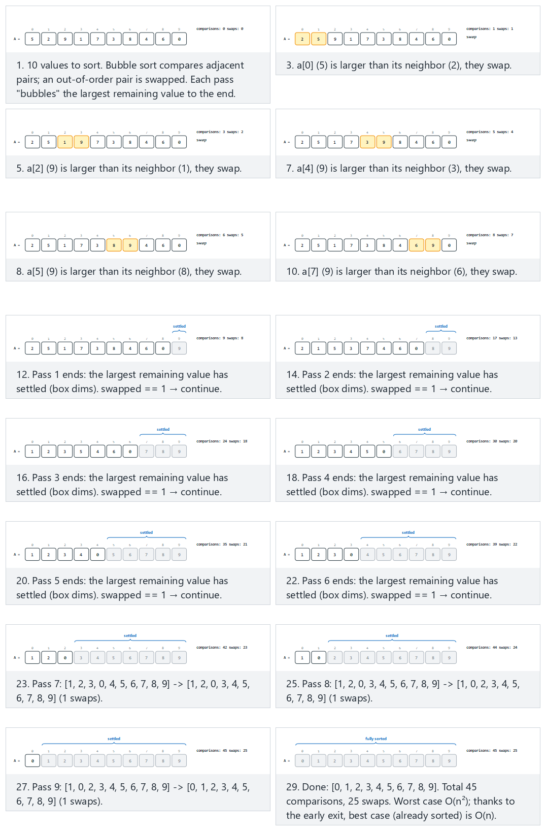
In the picker, also try already sorted — early exit (watch it stop after a single pass) and reverse sorted (the worst case: no early exit is ever possible), or press 🎲 for random data at four difficulty levels, or type your own array.
2.4 Try it
Full program: bubble_sort.c / BubbleSort.java
/* Week 10 -- Sorting
 * Bubble sort with early exit: repeatedly walk the array, swapping adjacent
 * out-of-order pairs; a pass with zero swaps means the array is already
 * sorted and the algorithm stops early. Prints the array after every pass
 * and the total comparisons/swaps.
 * CEN207 Data Structures (formerly CE205)
 */
#include <stdio.h>

static void print_array(const int a[], int n) {
    printf("[");
    for (int i = 0; i < n; i++) printf("%d%s", a[i], i + 1 < n ? ", " : "");
    printf("]\n");
}

void bubble_sort(int a[], int n, int *comparisons, int *swaps) {
    for (int pass = 0; pass < n - 1; pass++) {
        int swapped = 0;
        for (int i = 0; i < n - 1 - pass; i++) {
            (*comparisons)++;
            if (a[i] > a[i + 1]) {
                int tmp = a[i]; a[i] = a[i + 1]; a[i + 1] = tmp;
                (*swaps)++;
                swapped = 1;
            }
        }
        printf("  pass %d: ", pass + 1);
        print_array(a, n);
        if (!swapped) { printf("  no swaps this pass -> early exit\n"); break; }
    }
}

static void run_scenario(const char *label, int a[], int n) {
    printf("-- %s --\n", label);
    printf("before: ");
    print_array(a, n);
    int comparisons = 0, swaps = 0;
    bubble_sort(a, n, &comparisons, &swaps);
    printf("after:  ");
    print_array(a, n);
    printf("total: %d comparisons, %d swaps\n\n", comparisons, swaps);
}

int main(void) {
    int normal[] = {5, 2, 9, 1, 7, 3, 8, 4, 6, 0};
    int hard[] = {40, 11, 27, 8, 33, 16, 45, 2, 19, 37, 24, 6, 50, 29};
    int already_sorted[] = {1, 2, 3, 4, 5, 6, 7, 8, 9, 10, 11, 12};
    int reverse_sorted[] = {12, 11, 10, 9, 8, 7, 6, 5, 4, 3, 2, 1};

    run_scenario("normal: 10 unordered values", normal, 10);
    run_scenario("hard: 14 values, needs many passes", hard, 14);
    run_scenario("edge: already sorted -- early exit after one pass", already_sorted, 12);
    run_scenario("edge: reverse sorted -- worst case, no early exit", reverse_sorted, 12);

    return 0;
}
/* Week 10 -- Sorting
 * Bubble sort with early exit: repeatedly walk the array, swapping adjacent
 * out-of-order pairs; a pass with zero swaps means the array is already
 * sorted and the algorithm stops early. Prints the array after every pass
 * and the total comparisons/swaps.
 * CEN207 Data Structures (formerly CE205)
 */
public class BubbleSort {
    static int comparisons, swaps;

    static void printArray(int[] a) {
        StringBuilder sb = new StringBuilder("[");
        for (int i = 0; i < a.length; i++) { sb.append(a[i]); if (i + 1 < a.length) sb.append(", "); }
        sb.append(']');
        System.out.println(sb);
    }

    static void bubbleSort(int[] a) {
        int n = a.length;
        for (int pass = 0; pass < n - 1; pass++) {
            boolean swapped = false;
            for (int i = 0; i < n - 1 - pass; i++) {
                comparisons++;
                if (a[i] > a[i + 1]) {
                    int tmp = a[i]; a[i] = a[i + 1]; a[i + 1] = tmp;
                    swaps++;
                    swapped = true;
                }
            }
            System.out.print("  pass " + (pass + 1) + ": ");
            printArray(a);
            if (!swapped) { System.out.println("  no swaps this pass -> early exit"); break; }
        }
    }

    static void runScenario(String label, int[] a) {
        System.out.println("-- " + label + " --");
        System.out.print("before: ");
        printArray(a);
        comparisons = 0; swaps = 0;
        bubbleSort(a);
        System.out.print("after:  ");
        printArray(a);
        System.out.println("total: " + comparisons + " comparisons, " + swaps + " swaps");
        System.out.println();
    }

    public static void main(String[] args) {
        int[] normal = {5, 2, 9, 1, 7, 3, 8, 4, 6, 0};
        int[] hard = {40, 11, 27, 8, 33, 16, 45, 2, 19, 37, 24, 6, 50, 29};
        int[] alreadySorted = {1, 2, 3, 4, 5, 6, 7, 8, 9, 10, 11, 12};
        int[] reverseSorted = {12, 11, 10, 9, 8, 7, 6, 5, 4, 3, 2, 1};

        runScenario("normal: 10 unordered values", normal);
        runScenario("hard: 14 values, needs many passes", hard);
        runScenario("edge: already sorted -- early exit after one pass", alreadySorted);
        runScenario("edge: reverse sorted -- worst case, no early exit", reverseSorted);
    }
}
Try it
Expected output:
-- normal: 10 unordered values --
before: [5, 2, 9, 1, 7, 3, 8, 4, 6, 0]
  pass 1: [2, 5, 1, 7, 3, 8, 4, 6, 0, 9]
  pass 2: [2, 1, 5, 3, 7, 4, 6, 0, 8, 9]
  pass 3: [1, 2, 3, 5, 4, 6, 0, 7, 8, 9]
  pass 4: [1, 2, 3, 4, 5, 0, 6, 7, 8, 9]
  pass 5: [1, 2, 3, 4, 0, 5, 6, 7, 8, 9]
  pass 6: [1, 2, 3, 0, 4, 5, 6, 7, 8, 9]
  pass 7: [1, 2, 0, 3, 4, 5, 6, 7, 8, 9]
  pass 8: [1, 0, 2, 3, 4, 5, 6, 7, 8, 9]
  pass 9: [0, 1, 2, 3, 4, 5, 6, 7, 8, 9]
after:  [0, 1, 2, 3, 4, 5, 6, 7, 8, 9]
total: 45 comparisons, 25 swaps

-- hard: 14 values, needs many passes --
before: [40, 11, 27, 8, 33, 16, 45, 2, 19, 37, 24, 6, 50, 29]
  pass 1: [11, 27, 8, 33, 16, 40, 2, 19, 37, 24, 6, 45, 29, 50]
  pass 2: [11, 8, 27, 16, 33, 2, 19, 37, 24, 6, 40, 29, 45, 50]
  pass 3: [8, 11, 16, 27, 2, 19, 33, 24, 6, 37, 29, 40, 45, 50]
  pass 4: [8, 11, 16, 2, 19, 27, 24, 6, 33, 29, 37, 40, 45, 50]
  pass 5: [8, 11, 2, 16, 19, 24, 6, 27, 29, 33, 37, 40, 45, 50]
  pass 6: [8, 2, 11, 16, 19, 6, 24, 27, 29, 33, 37, 40, 45, 50]
  pass 7: [2, 8, 11, 16, 6, 19, 24, 27, 29, 33, 37, 40, 45, 50]
  pass 8: [2, 8, 11, 6, 16, 19, 24, 27, 29, 33, 37, 40, 45, 50]
  pass 9: [2, 8, 6, 11, 16, 19, 24, 27, 29, 33, 37, 40, 45, 50]
  pass 10: [2, 6, 8, 11, 16, 19, 24, 27, 29, 33, 37, 40, 45, 50]
  pass 11: [2, 6, 8, 11, 16, 19, 24, 27, 29, 33, 37, 40, 45, 50]
  no swaps this pass -> early exit
after:  [2, 6, 8, 11, 16, 19, 24, 27, 29, 33, 37, 40, 45, 50]
total: 88 comparisons, 42 swaps

-- edge: already sorted -- early exit after one pass --
before: [1, 2, 3, 4, 5, 6, 7, 8, 9, 10, 11, 12]
  pass 1: [1, 2, 3, 4, 5, 6, 7, 8, 9, 10, 11, 12]
  no swaps this pass -> early exit
after:  [1, 2, 3, 4, 5, 6, 7, 8, 9, 10, 11, 12]
total: 11 comparisons, 0 swaps

-- edge: reverse sorted -- worst case, no early exit --
before: [12, 11, 10, 9, 8, 7, 6, 5, 4, 3, 2, 1]
  pass 1: [11, 10, 9, 8, 7, 6, 5, 4, 3, 2, 1, 12]
  pass 2: [10, 9, 8, 7, 6, 5, 4, 3, 2, 1, 11, 12]
  pass 3: [9, 8, 7, 6, 5, 4, 3, 2, 1, 10, 11, 12]
  pass 4: [8, 7, 6, 5, 4, 3, 2, 1, 9, 10, 11, 12]
  pass 5: [7, 6, 5, 4, 3, 2, 1, 8, 9, 10, 11, 12]
  pass 6: [6, 5, 4, 3, 2, 1, 7, 8, 9, 10, 11, 12]
  pass 7: [5, 4, 3, 2, 1, 6, 7, 8, 9, 10, 11, 12]
  pass 8: [4, 3, 2, 1, 5, 6, 7, 8, 9, 10, 11, 12]
  pass 9: [3, 2, 1, 4, 5, 6, 7, 8, 9, 10, 11, 12]
  pass 10: [2, 1, 3, 4, 5, 6, 7, 8, 9, 10, 11, 12]
  pass 11: [1, 2, 3, 4, 5, 6, 7, 8, 9, 10, 11, 12]
after:  [1, 2, 3, 4, 5, 6, 7, 8, 9, 10, 11, 12]
total: 66 comparisons, 66 swaps
2.5 Complexity, mistakes, self-check
Complexity. Best case O(n) (already sorted: one pass, n-1 comparisons, the early exit fires immediately). Worst case and average case both O(n^2) (reverse-sorted or random input: roughly n^2/2 comparisons and, on average, n^2/4 swaps). Space: O(1), in place. Bubble sort is stable: it only swaps strictly out-of-order neighbors (a[i] > a[i+1]), so two equal elements are never swapped past each other.
Common mistakes
- Forgetting the early-exit flag entirely. Without it, bubble sort is always
O(n^2), even on data that is already sorted — the single change that makes it worth teaching at all is exactly this flag. - Shrinking the wrong end of the inner loop. After
passfull passes, the lastpasselements are guaranteed settled (each pass bubbles one more maximum into place from the right), so the inner loop must shrink ton - 1 - pass, not stay fixed atn - 1— the latter still works, just re-compares already-settled elements for no reason, silently degrading an already-inefficient algorithm further. - Using
>=instead of>in the swap condition.a[i] >= a[i+1]would swap equal elements too, destroying stability for no benefit — always use strict>for an ascending stable bubble sort.
Self-check: best case vs. worst case
Explain, in one sentence each, why bubble sort's best case is O(n) and why its worst case is O(n^2), using the early-exit flag in your answer for the best case.
Answer. Best case: on an already-sorted array, the very first pass makes zero swaps (every adjacent pair is already in order), so swapped stays 0, the early exit fires, and only n-1 comparisons ever happen — O(n). Worst case: on a reverse-sorted array, every single pass finds every remaining pair out of order, so no pass ever exits early, and the algorithm runs all n-1 passes, each shrinking by one, giving (n-1) + (n-2) + ... + 1 = n(n-1)/2 comparisons — O(n^2).
3. Selection sort
3.1 A question to start
Bubble sort's small, local swaps add up to a lot of data movement — section 2's "reverse sorted" scenario did 66 swaps to sort 12 values. What if, instead, you found the single smallest remaining value with a full scan, and moved it directly to its final position in one swap? You would still need to scan the whole unsorted region every time (no early exit is possible — you cannot know an element is the minimum without checking every candidate), but you would swap far less. That trade — full scans, but minimal writes — is selection sort. Like bubble sort, it has no single named inventor; it is the direct algorithmic expression of "repeatedly pick the smallest remaining item," an idea at least as old as sorting itself.
3.2 The idea: find the minimum, swap it into place
For each position i from 0 to n-2, scan the remainder of the array (i+1 to n-1) to find the index of its minimum value, min_idx. Once the scan finishes, swap a[i] and a[min_idx] — but only if min_idx != i; if position i already held the minimum, skip the pointless swap. The sorted region grows from the left this time (the opposite of bubble sort's right-growing sorted tail), because each step fixes the final value of position i for good before moving on to i+1.
3.3 In memory, and the code
void selection_sort(int a[], int n, int *comparisons, int *swaps) {
    for (int i = 0; i < n - 1; i++) {
        int min_idx = i;
        for (int j = i + 1; j < n; j++) {
            (*comparisons)++;
            if (a[j] < a[min_idx]) min_idx = j;
        }
        if (min_idx != i) {              /* skip the swap if i is already the minimum */
            int tmp = a[i];
            a[i] = a[min_idx];
            a[min_idx] = tmp;
            (*swaps)++;
        }
    }
}
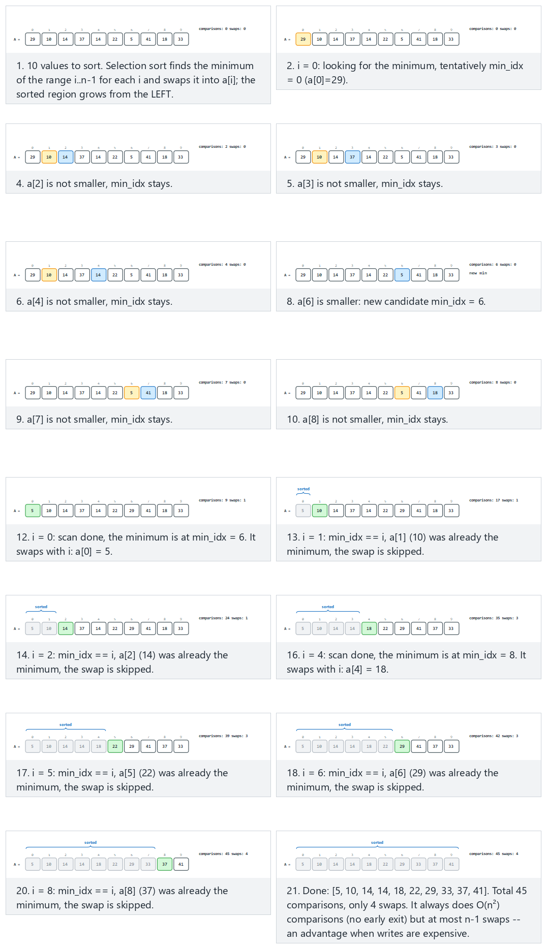
In the picker, also try duplicates — ties keep the first minimum found and already sorted — a full scan still happens for every i (there is no early exit here, unlike bubble sort), or press 🎲 for random data, or type your own array.
3.4 Try it
Full program: selection_sort.c / SelectionSort.java
/* Week 10 -- Sorting
 * Selection sort: for each position i, scan the unsorted remainder for its
 * minimum and swap it into place. The sorted region grows on the LEFT; at
 * most n-1 swaps ever happen, but every position still does a full scan
 * (no early exit). Prints the array after every position and the total
 * comparisons/swaps.
 * CEN207 Data Structures (formerly CE205)
 */
#include <stdio.h>

static void print_array(const int a[], int n) {
    printf("[");
    for (int i = 0; i < n; i++) printf("%d%s", a[i], i + 1 < n ? ", " : "");
    printf("]\n");
}

void selection_sort(int a[], int n, int *comparisons, int *swaps) {
    for (int i = 0; i < n - 1; i++) {
        int min_idx = i;
        for (int j = i + 1; j < n; j++) {
            (*comparisons)++;
            if (a[j] < a[min_idx]) min_idx = j;
        }
        if (min_idx != i) {
            int tmp = a[i]; a[i] = a[min_idx]; a[min_idx] = tmp;
            (*swaps)++;
        }
        printf("  i=%d: min_idx=%d -> ", i, min_idx);
        print_array(a, n);
    }
}

static void run_scenario(const char *label, int a[], int n) {
    printf("-- %s --\n", label);
    printf("before: ");
    print_array(a, n);
    int comparisons = 0, swaps = 0;
    selection_sort(a, n, &comparisons, &swaps);
    printf("after:  ");
    print_array(a, n);
    printf("total: %d comparisons, %d swaps\n\n", comparisons, swaps);
}

int main(void) {
    int normal[] = {29, 10, 14, 37, 14, 22, 5, 41, 18, 33};
    int hard[] = {50, 3, 47, 8, 44, 12, 39, 16, 34, 20, 29, 24, 25, 27};
    int already_sorted[] = {1, 2, 3, 4, 5, 6, 7, 8, 9, 10, 11, 12};
    int reverse_sorted[] = {12, 11, 10, 9, 8, 7, 6, 5, 4, 3, 2, 1};

    run_scenario("normal: 10 unordered values", normal, 10);
    run_scenario("hard: 14 values, the minimum keeps moving", hard, 14);
    run_scenario("edge: already sorted -- a full scan still happens for every i", already_sorted, 12);
    run_scenario("edge: reverse sorted -- every step swaps", reverse_sorted, 12);

    return 0;
}
/* Week 10 -- Sorting
 * Selection sort: for each position i, scan the unsorted remainder for its
 * minimum and swap it into place. The sorted region grows on the LEFT; at
 * most n-1 swaps ever happen, but every position still does a full scan
 * (no early exit). Prints the array after every position and the total
 * comparisons/swaps.
 * CEN207 Data Structures (formerly CE205)
 */
public class SelectionSort {
    static int comparisons, swaps;

    static void printArray(int[] a) {
        StringBuilder sb = new StringBuilder("[");
        for (int i = 0; i < a.length; i++) { sb.append(a[i]); if (i + 1 < a.length) sb.append(", "); }
        sb.append(']');
        System.out.println(sb);
    }

    static void selectionSort(int[] a) {
        int n = a.length;
        for (int i = 0; i < n - 1; i++) {
            int minIdx = i;
            for (int j = i + 1; j < n; j++) {
                comparisons++;
                if (a[j] < a[minIdx]) minIdx = j;
            }
            if (minIdx != i) {
                int tmp = a[i]; a[i] = a[minIdx]; a[minIdx] = tmp;
                swaps++;
            }
            System.out.print("  i=" + i + ": min_idx=" + minIdx + " -> ");
            printArray(a);
        }
    }

    static void runScenario(String label, int[] a) {
        System.out.println("-- " + label + " --");
        System.out.print("before: ");
        printArray(a);
        comparisons = 0; swaps = 0;
        selectionSort(a);
        System.out.print("after:  ");
        printArray(a);
        System.out.println("total: " + comparisons + " comparisons, " + swaps + " swaps");
        System.out.println();
    }

    public static void main(String[] args) {
        int[] normal = {29, 10, 14, 37, 14, 22, 5, 41, 18, 33};
        int[] hard = {50, 3, 47, 8, 44, 12, 39, 16, 34, 20, 29, 24, 25, 27};
        int[] alreadySorted = {1, 2, 3, 4, 5, 6, 7, 8, 9, 10, 11, 12};
        int[] reverseSorted = {12, 11, 10, 9, 8, 7, 6, 5, 4, 3, 2, 1};

        runScenario("normal: 10 unordered values", normal);
        runScenario("hard: 14 values, the minimum keeps moving", hard);
        runScenario("edge: already sorted -- a full scan still happens for every i", alreadySorted);
        runScenario("edge: reverse sorted -- every step swaps", reverseSorted);
    }
}
Try it
Expected output:
-- normal: 10 unordered values --
before: [29, 10, 14, 37, 14, 22, 5, 41, 18, 33]
  i=0: min_idx=6 -> [5, 10, 14, 37, 14, 22, 29, 41, 18, 33]
  i=1: min_idx=1 -> [5, 10, 14, 37, 14, 22, 29, 41, 18, 33]
  i=2: min_idx=2 -> [5, 10, 14, 37, 14, 22, 29, 41, 18, 33]
  i=3: min_idx=4 -> [5, 10, 14, 14, 37, 22, 29, 41, 18, 33]
  i=4: min_idx=8 -> [5, 10, 14, 14, 18, 22, 29, 41, 37, 33]
  i=5: min_idx=5 -> [5, 10, 14, 14, 18, 22, 29, 41, 37, 33]
  i=6: min_idx=6 -> [5, 10, 14, 14, 18, 22, 29, 41, 37, 33]
  i=7: min_idx=9 -> [5, 10, 14, 14, 18, 22, 29, 33, 37, 41]
  i=8: min_idx=8 -> [5, 10, 14, 14, 18, 22, 29, 33, 37, 41]
after:  [5, 10, 14, 14, 18, 22, 29, 33, 37, 41]
total: 45 comparisons, 4 swaps

-- hard: 14 values, the minimum keeps moving --
before: [50, 3, 47, 8, 44, 12, 39, 16, 34, 20, 29, 24, 25, 27]
  i=0: min_idx=1 -> [3, 50, 47, 8, 44, 12, 39, 16, 34, 20, 29, 24, 25, 27]
  i=1: min_idx=3 -> [3, 8, 47, 50, 44, 12, 39, 16, 34, 20, 29, 24, 25, 27]
  i=2: min_idx=5 -> [3, 8, 12, 50, 44, 47, 39, 16, 34, 20, 29, 24, 25, 27]
  i=3: min_idx=7 -> [3, 8, 12, 16, 44, 47, 39, 50, 34, 20, 29, 24, 25, 27]
  i=4: min_idx=9 -> [3, 8, 12, 16, 20, 47, 39, 50, 34, 44, 29, 24, 25, 27]
  i=5: min_idx=11 -> [3, 8, 12, 16, 20, 24, 39, 50, 34, 44, 29, 47, 25, 27]
  i=6: min_idx=12 -> [3, 8, 12, 16, 20, 24, 25, 50, 34, 44, 29, 47, 39, 27]
  i=7: min_idx=13 -> [3, 8, 12, 16, 20, 24, 25, 27, 34, 44, 29, 47, 39, 50]
  i=8: min_idx=10 -> [3, 8, 12, 16, 20, 24, 25, 27, 29, 44, 34, 47, 39, 50]
  i=9: min_idx=10 -> [3, 8, 12, 16, 20, 24, 25, 27, 29, 34, 44, 47, 39, 50]
  i=10: min_idx=12 -> [3, 8, 12, 16, 20, 24, 25, 27, 29, 34, 39, 47, 44, 50]
  i=11: min_idx=12 -> [3, 8, 12, 16, 20, 24, 25, 27, 29, 34, 39, 44, 47, 50]
  i=12: min_idx=12 -> [3, 8, 12, 16, 20, 24, 25, 27, 29, 34, 39, 44, 47, 50]
after:  [3, 8, 12, 16, 20, 24, 25, 27, 29, 34, 39, 44, 47, 50]
total: 91 comparisons, 12 swaps

-- edge: already sorted -- a full scan still happens for every i --
before: [1, 2, 3, 4, 5, 6, 7, 8, 9, 10, 11, 12]
  i=0: min_idx=0 -> [1, 2, 3, 4, 5, 6, 7, 8, 9, 10, 11, 12]
  i=1: min_idx=1 -> [1, 2, 3, 4, 5, 6, 7, 8, 9, 10, 11, 12]
  i=2: min_idx=2 -> [1, 2, 3, 4, 5, 6, 7, 8, 9, 10, 11, 12]
  i=3: min_idx=3 -> [1, 2, 3, 4, 5, 6, 7, 8, 9, 10, 11, 12]
  i=4: min_idx=4 -> [1, 2, 3, 4, 5, 6, 7, 8, 9, 10, 11, 12]
  i=5: min_idx=5 -> [1, 2, 3, 4, 5, 6, 7, 8, 9, 10, 11, 12]
  i=6: min_idx=6 -> [1, 2, 3, 4, 5, 6, 7, 8, 9, 10, 11, 12]
  i=7: min_idx=7 -> [1, 2, 3, 4, 5, 6, 7, 8, 9, 10, 11, 12]
  i=8: min_idx=8 -> [1, 2, 3, 4, 5, 6, 7, 8, 9, 10, 11, 12]
  i=9: min_idx=9 -> [1, 2, 3, 4, 5, 6, 7, 8, 9, 10, 11, 12]
  i=10: min_idx=10 -> [1, 2, 3, 4, 5, 6, 7, 8, 9, 10, 11, 12]
after:  [1, 2, 3, 4, 5, 6, 7, 8, 9, 10, 11, 12]
total: 66 comparisons, 0 swaps

-- edge: reverse sorted -- every step swaps --
before: [12, 11, 10, 9, 8, 7, 6, 5, 4, 3, 2, 1]
  i=0: min_idx=11 -> [1, 11, 10, 9, 8, 7, 6, 5, 4, 3, 2, 12]
  i=1: min_idx=10 -> [1, 2, 10, 9, 8, 7, 6, 5, 4, 3, 11, 12]
  i=2: min_idx=9 -> [1, 2, 3, 9, 8, 7, 6, 5, 4, 10, 11, 12]
  i=3: min_idx=8 -> [1, 2, 3, 4, 8, 7, 6, 5, 9, 10, 11, 12]
  i=4: min_idx=7 -> [1, 2, 3, 4, 5, 7, 6, 8, 9, 10, 11, 12]
  i=5: min_idx=6 -> [1, 2, 3, 4, 5, 6, 7, 8, 9, 10, 11, 12]
  i=6: min_idx=6 -> [1, 2, 3, 4, 5, 6, 7, 8, 9, 10, 11, 12]
  i=7: min_idx=7 -> [1, 2, 3, 4, 5, 6, 7, 8, 9, 10, 11, 12]
  i=8: min_idx=8 -> [1, 2, 3, 4, 5, 6, 7, 8, 9, 10, 11, 12]
  i=9: min_idx=9 -> [1, 2, 3, 4, 5, 6, 7, 8, 9, 10, 11, 12]
  i=10: min_idx=10 -> [1, 2, 3, 4, 5, 6, 7, 8, 9, 10, 11, 12]
after:  [1, 2, 3, 4, 5, 6, 7, 8, 9, 10, 11, 12]
total: 66 comparisons, 6 swaps
3.5 Complexity, mistakes, self-check
Complexity. Best, average, and worst case are all O(n^2) comparisons — always n(n-1)/2, regardless of input order, since the inner scan never has an early exit (you must check every remaining candidate to be sure you have the true minimum). But at most n-1 swaps, ever — far fewer than bubble sort's up to n(n-1)/2. Space: O(1), in place. Selection sort is NOT stable in general: the long-range swap that moves the minimum into position i can jump it past an equal-keyed element sitting in between (section 11 shows this happening on real data).
Common mistakes
- Swapping unconditionally, even when
min_idx == i. It is harmless for correctness but wastes a write every time the current position already holds the minimum — exactly the "few swaps" property that makes selection sort worth choosing over bubble sort in the first place, so skip it explicitly. - Expecting an early exit that does not exist. Unlike bubble sort, there is no flag to check here: finding the minimum of a range fundamentally requires examining every element in it, so selection sort is
O(n^2)even on already-sorted input — confirm this in the "already sorted" example above (66 comparisons, the fulln(n-1)/2, forn = 12). - Assuming selection sort is stable because it "looks simple". It is one of the two clearest unstable sorts this week (along with quick sort); see section 11 for a worked example of exactly how a tie gets reordered.
Self-check: why selection sort minimizes swaps
Selection sort does at most n-1 swaps total. Explain why that bound holds regardless of the input, and contrast it with bubble sort's worst case of n(n-1)/2 swaps.
Answer. Selection sort performs at most one swap per iteration of the outer loop — and only when min_idx != i — and the outer loop runs n-1 times, so the total can never exceed n-1, no matter how scrambled the input is; every element that needs to move at all moves in one single swap directly to its final resting place. Bubble sort, in contrast, moves an out-of-place element one position at a time on each pass, so a value that starts at the wrong end of the array (like the 1 in section 2's reverse-sorted example) needs many separate adjacent swaps to travel all the way across — up to n(n-1)/2 of them in total across the whole sort.
4. Insertion sort
4.1 A question to start
Think about how you sort a hand of playing cards. You do not compare every card against every other card the way bubble or selection sort does. You hold a small sorted hand in your left hand, pick up the next card with your right, and slide it into the one gap where it belongs, shifting the cards in between one space over. That is exactly insertion sort — and it is the sort you will draw, by hand, on the board every time this course needs a quick example, because it is the one whose picture matches how people actually sort things.
4.2 The idea, drawn the way you will draw it
Insertion sort maintains the invariant that A[0..i-1] is already sorted. At each step i, it pulls out A[i] as the key — set it aside, out of the array, the way you would lift a card out of your hand — and then compares the key against the sorted prefix from the right: while the element just to the key's left is greater than the key, shift that element one cell to the right (opening a "hole" that moves left with every shift), and move the comparison point one further left. The moment you find an element that is not greater than the key (or you run off the left end of the array), the hole is the key's correct spot — drop it in.
This is drawn, on the board, exactly like this — and the animation below draws it the same way:
- a brace over
A[0..i-1]labeled "already sorted", growing by one element every outer-loop step; - the key pulled out of the array and shown in a separate red box above its old position — it is not part of the array while it is being compared, exactly like a card held in your other hand;
- the region being scanned splits in two on the fly: elements confirmed
<= key(the scan has not reached them, or it stopped there) stay put; elements found> keyshift one cell right, opening the hole; - a shift arrow from the shifting element's old cell to its new cell, so the eye follows the hole moving left one step at a time;
- once a comparison finds
a[j] <= key, the loop stops and the key drops into the hole — the red box disappears and a plain array cell appears in its place.
4.3 In memory, and the code
void insertion_sort(int a[], int n, int *comparisons, int *shifts) {
    for (int i = 1; i < n; i++) {
        int key = a[i];               /* pull the key out (the red box) */
        int j = i - 1;
        while (j >= 0 && a[j] > key) {
            a[j + 1] = a[j];           /* shift right, opening a hole at j */
            j--;
        }
        a[j + 1] = key;                /* the key drops into the hole */
    }
}
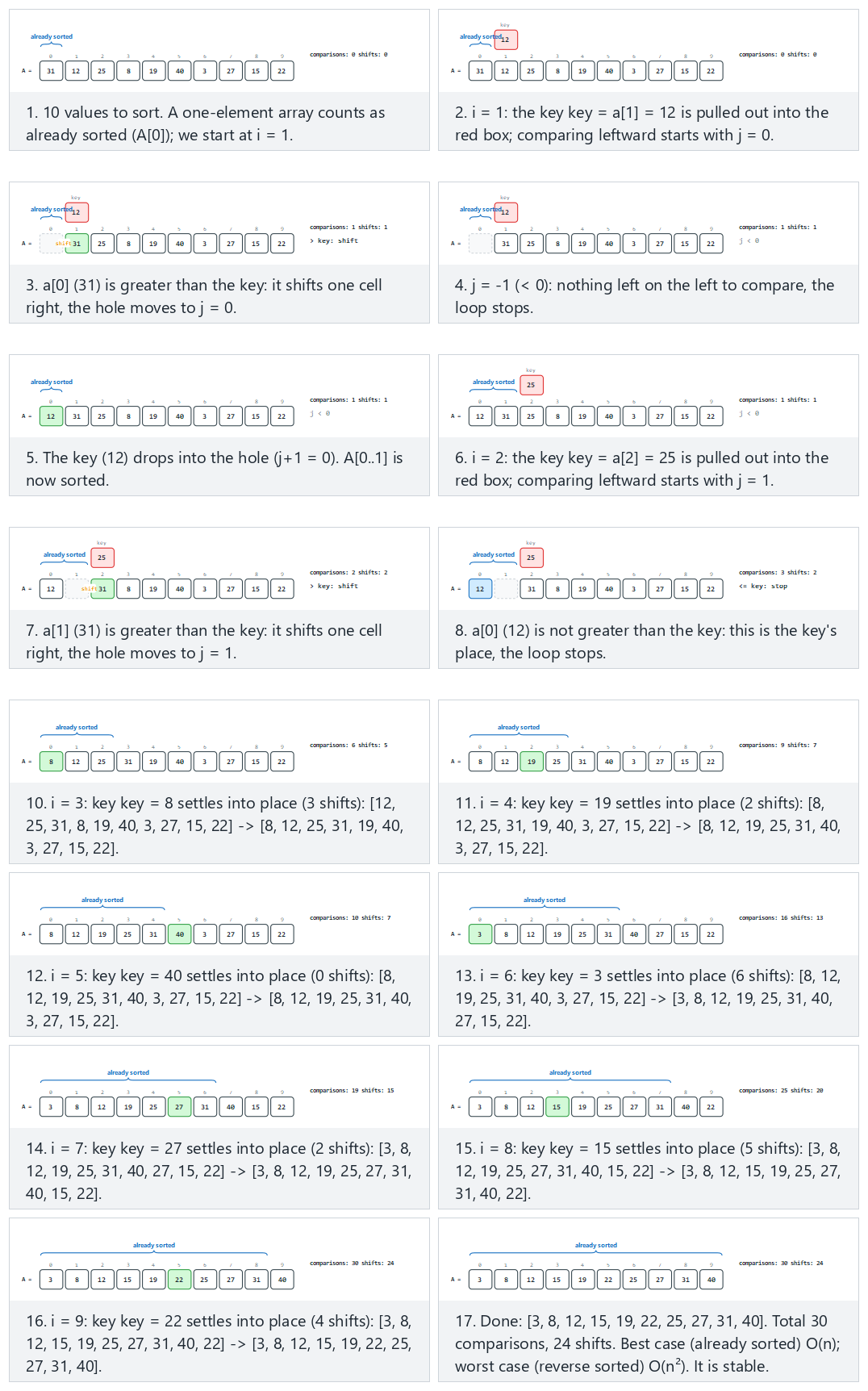
In the picker, also try duplicates — a tie stops the shift (stable) and reverse sorted — worst case, every key shifts to the front, or press 🎲 for random data, or type your own array. Compare what you see here against your own board notes from earlier in the course — this animation is drawn to match exactly.
4.4 Try it
Full program: insertion_sort.c / InsertionSort.java
/* Week 10 -- Sorting
 * Insertion sort: for each i, pull out a[i] as the key, then shift every
 * element greater than the key one cell right until the key's correct spot
 * (its "hole") is found. Prints the key and the array after every
 * insertion, plus total comparisons/shifts.
 * CEN207 Data Structures (formerly CE205)
 */
#include <stdio.h>

static void print_array(const int a[], int n) {
    printf("[");
    for (int i = 0; i < n; i++) printf("%d%s", a[i], i + 1 < n ? ", " : "");
    printf("]\n");
}

void insertion_sort(int a[], int n, int *comparisons, int *shifts) {
    for (int i = 1; i < n; i++) {
        int key = a[i];
        int j = i - 1;
        while (j >= 0) {
            (*comparisons)++;
            if (a[j] <= key) break;
            a[j + 1] = a[j];
            (*shifts)++;
            j--;
        }
        a[j + 1] = key;
        printf("  i=%d: key=%d -> ", i, key);
        print_array(a, n);
    }
}

static void run_scenario(const char *label, int a[], int n) {
    printf("-- %s --\n", label);
    printf("before: ");
    print_array(a, n);
    int comparisons = 0, shifts = 0;
    insertion_sort(a, n, &comparisons, &shifts);
    printf("after:  ");
    print_array(a, n);
    printf("total: %d comparisons, %d shifts\n\n", comparisons, shifts);
}

int main(void) {
    int normal[] = {31, 12, 25, 8, 19, 40, 3, 27, 15, 22};
    int hard[] = {45, 2, 38, 9, 33, 14, 29, 6, 41, 18, 24, 11, 36, 20};
    int already_sorted[] = {1, 2, 3, 4, 5, 6, 7, 8, 9, 10, 11, 12};
    int reverse_sorted[] = {12, 11, 10, 9, 8, 7, 6, 5, 4, 3, 2, 1};

    run_scenario("normal: 10 unordered values", normal, 10);
    run_scenario("hard: 14 values, needs long shifts", hard, 14);
    run_scenario("edge: already sorted -- one comparison per i, zero shifts", already_sorted, 12);
    run_scenario("edge: reverse sorted -- worst case, every key shifts to the front", reverse_sorted, 12);

    return 0;
}
/* Week 10 -- Sorting
 * Insertion sort: for each i, pull out a[i] as the key, then shift every
 * element greater than the key one cell right until the key's correct spot
 * (its "hole") is found. Prints the key and the array after every
 * insertion, plus total comparisons/shifts.
 * CEN207 Data Structures (formerly CE205)
 */
public class InsertionSort {
    static int comparisons, shifts;

    static void printArray(int[] a) {
        StringBuilder sb = new StringBuilder("[");
        for (int i = 0; i < a.length; i++) { sb.append(a[i]); if (i + 1 < a.length) sb.append(", "); }
        sb.append(']');
        System.out.println(sb);
    }

    static void insertionSort(int[] a) {
        int n = a.length;
        for (int i = 1; i < n; i++) {
            int key = a[i];
            int j = i - 1;
            while (j >= 0) {
                comparisons++;
                if (a[j] <= key) break;
                a[j + 1] = a[j];
                shifts++;
                j--;
            }
            a[j + 1] = key;
            System.out.print("  i=" + i + ": key=" + key + " -> ");
            printArray(a);
        }
    }

    static void runScenario(String label, int[] a) {
        System.out.println("-- " + label + " --");
        System.out.print("before: ");
        printArray(a);
        comparisons = 0; shifts = 0;
        insertionSort(a);
        System.out.print("after:  ");
        printArray(a);
        System.out.println("total: " + comparisons + " comparisons, " + shifts + " shifts");
        System.out.println();
    }

    public static void main(String[] args) {
        int[] normal = {31, 12, 25, 8, 19, 40, 3, 27, 15, 22};
        int[] hard = {45, 2, 38, 9, 33, 14, 29, 6, 41, 18, 24, 11, 36, 20};
        int[] alreadySorted = {1, 2, 3, 4, 5, 6, 7, 8, 9, 10, 11, 12};
        int[] reverseSorted = {12, 11, 10, 9, 8, 7, 6, 5, 4, 3, 2, 1};

        runScenario("normal: 10 unordered values", normal);
        runScenario("hard: 14 values, needs long shifts", hard);
        runScenario("edge: already sorted -- one comparison per i, zero shifts", alreadySorted);
        runScenario("edge: reverse sorted -- worst case, every key shifts to the front", reverseSorted);
    }
}
Try it
Expected output:
-- normal: 10 unordered values --
before: [31, 12, 25, 8, 19, 40, 3, 27, 15, 22]
  i=1: key=12 -> [12, 31, 25, 8, 19, 40, 3, 27, 15, 22]
  i=2: key=25 -> [12, 25, 31, 8, 19, 40, 3, 27, 15, 22]
  i=3: key=8 -> [8, 12, 25, 31, 19, 40, 3, 27, 15, 22]
  i=4: key=19 -> [8, 12, 19, 25, 31, 40, 3, 27, 15, 22]
  i=5: key=40 -> [8, 12, 19, 25, 31, 40, 3, 27, 15, 22]
  i=6: key=3 -> [3, 8, 12, 19, 25, 31, 40, 27, 15, 22]
  i=7: key=27 -> [3, 8, 12, 19, 25, 27, 31, 40, 15, 22]
  i=8: key=15 -> [3, 8, 12, 15, 19, 25, 27, 31, 40, 22]
  i=9: key=22 -> [3, 8, 12, 15, 19, 22, 25, 27, 31, 40]
after:  [3, 8, 12, 15, 19, 22, 25, 27, 31, 40]
total: 30 comparisons, 24 shifts

-- hard: 14 values, needs long shifts --
before: [45, 2, 38, 9, 33, 14, 29, 6, 41, 18, 24, 11, 36, 20]
  i=1: key=2 -> [2, 45, 38, 9, 33, 14, 29, 6, 41, 18, 24, 11, 36, 20]
  i=2: key=38 -> [2, 38, 45, 9, 33, 14, 29, 6, 41, 18, 24, 11, 36, 20]
  i=3: key=9 -> [2, 9, 38, 45, 33, 14, 29, 6, 41, 18, 24, 11, 36, 20]
  i=4: key=33 -> [2, 9, 33, 38, 45, 14, 29, 6, 41, 18, 24, 11, 36, 20]
  i=5: key=14 -> [2, 9, 14, 33, 38, 45, 29, 6, 41, 18, 24, 11, 36, 20]
  i=6: key=29 -> [2, 9, 14, 29, 33, 38, 45, 6, 41, 18, 24, 11, 36, 20]
  i=7: key=6 -> [2, 6, 9, 14, 29, 33, 38, 45, 41, 18, 24, 11, 36, 20]
  i=8: key=41 -> [2, 6, 9, 14, 29, 33, 38, 41, 45, 18, 24, 11, 36, 20]
  i=9: key=18 -> [2, 6, 9, 14, 18, 29, 33, 38, 41, 45, 24, 11, 36, 20]
  i=10: key=24 -> [2, 6, 9, 14, 18, 24, 29, 33, 38, 41, 45, 11, 36, 20]
  i=11: key=11 -> [2, 6, 9, 11, 14, 18, 24, 29, 33, 38, 41, 45, 36, 20]
  i=12: key=36 -> [2, 6, 9, 11, 14, 18, 24, 29, 33, 36, 38, 41, 45, 20]
  i=13: key=20 -> [2, 6, 9, 11, 14, 18, 20, 24, 29, 33, 36, 38, 41, 45]
after:  [2, 6, 9, 11, 14, 18, 20, 24, 29, 33, 36, 38, 41, 45]
total: 59 comparisons, 47 shifts

-- edge: already sorted -- one comparison per i, zero shifts --
before: [1, 2, 3, 4, 5, 6, 7, 8, 9, 10, 11, 12]
  i=1: key=2 -> [1, 2, 3, 4, 5, 6, 7, 8, 9, 10, 11, 12]
  i=2: key=3 -> [1, 2, 3, 4, 5, 6, 7, 8, 9, 10, 11, 12]
  i=3: key=4 -> [1, 2, 3, 4, 5, 6, 7, 8, 9, 10, 11, 12]
  i=4: key=5 -> [1, 2, 3, 4, 5, 6, 7, 8, 9, 10, 11, 12]
  i=5: key=6 -> [1, 2, 3, 4, 5, 6, 7, 8, 9, 10, 11, 12]
  i=6: key=7 -> [1, 2, 3, 4, 5, 6, 7, 8, 9, 10, 11, 12]
  i=7: key=8 -> [1, 2, 3, 4, 5, 6, 7, 8, 9, 10, 11, 12]
  i=8: key=9 -> [1, 2, 3, 4, 5, 6, 7, 8, 9, 10, 11, 12]
  i=9: key=10 -> [1, 2, 3, 4, 5, 6, 7, 8, 9, 10, 11, 12]
  i=10: key=11 -> [1, 2, 3, 4, 5, 6, 7, 8, 9, 10, 11, 12]
  i=11: key=12 -> [1, 2, 3, 4, 5, 6, 7, 8, 9, 10, 11, 12]
after:  [1, 2, 3, 4, 5, 6, 7, 8, 9, 10, 11, 12]
total: 11 comparisons, 0 shifts

-- edge: reverse sorted -- worst case, every key shifts to the front --
before: [12, 11, 10, 9, 8, 7, 6, 5, 4, 3, 2, 1]
  i=1: key=11 -> [11, 12, 10, 9, 8, 7, 6, 5, 4, 3, 2, 1]
  i=2: key=10 -> [10, 11, 12, 9, 8, 7, 6, 5, 4, 3, 2, 1]
  i=3: key=9 -> [9, 10, 11, 12, 8, 7, 6, 5, 4, 3, 2, 1]
  i=4: key=8 -> [8, 9, 10, 11, 12, 7, 6, 5, 4, 3, 2, 1]
  i=5: key=7 -> [7, 8, 9, 10, 11, 12, 6, 5, 4, 3, 2, 1]
  i=6: key=6 -> [6, 7, 8, 9, 10, 11, 12, 5, 4, 3, 2, 1]
  i=7: key=5 -> [5, 6, 7, 8, 9, 10, 11, 12, 4, 3, 2, 1]
  i=8: key=4 -> [4, 5, 6, 7, 8, 9, 10, 11, 12, 3, 2, 1]
  i=9: key=3 -> [3, 4, 5, 6, 7, 8, 9, 10, 11, 12, 2, 1]
  i=10: key=2 -> [2, 3, 4, 5, 6, 7, 8, 9, 10, 11, 12, 1]
  i=11: key=1 -> [1, 2, 3, 4, 5, 6, 7, 8, 9, 10, 11, 12]
after:  [1, 2, 3, 4, 5, 6, 7, 8, 9, 10, 11, 12]
total: 66 comparisons, 66 shifts
4.5 Complexity, mistakes, self-check
Complexity. Best case O(n) (already sorted: exactly one comparison per i, a[j] <= key is true immediately, zero shifts — confirmed above: 11 comparisons for n = 12, no more). Worst case O(n^2) (reverse sorted: every key must shift all the way to the front — confirmed above: 66 comparisons and 66 shifts, the full n(n-1)/2). Average case also O(n^2), but with a small constant factor that makes insertion sort genuinely fast in practice on small or nearly-sorted arrays — small enough that real-world library sorts (including C's qsort and Java's Arrays.sort for primitives) switch to insertion sort once a recursive quick/merge sort's sub-array shrinks below some threshold, typically around 16–32 elements. Space: O(1), in place. Insertion sort is stable: the shift condition is strict a[j] > key, so an element equal to the key is never shifted past it — the loop simply stops (see section 11 for a worked, tagged example).
Common mistakes
- Using
>=instead of>in the shift condition.a[j] >= keywould shift an equal element out of the way too, which still sorts correctly but destroys stability — always use strict>for a stable ascending insertion sort, exactly as this section's code does. - Forgetting the
j >= 0bound check, or checkinga[j] > keybeforej >= 0in the same condition (rather than after, short-circuited). If the key is the new minimum, the scan must run off the left end of the array; a comparison ordereda[j] > key && j >= 0readsa[-1]first, undefined behavior in C. Thewhile (j >= 0 && a[j] > key)order in this section's animation code (and thewhile (j >= 0) { if (a[j] <= key) break; ... }order used in the instrumented program above, which counts comparisons explicitly) both check the bound first — always check the index bound before the array access that depends on it. - Confusing insertion sort's growing sorted PREFIX with selection sort's. Both grow their sorted region from the left, but insertion sort's prefix is sorted because every new element gets inserted into its correct place inside it, while selection sort's prefix is sorted because every new position is filled with the correct value from a full scan of the remainder. The pictures look similar at first glance; the mechanism is opposite.
Self-check: why is insertion sort the natural choice for nearly-sorted data?
If an array is already sorted except for k elements that are each only a short distance from their final position, argue informally why insertion sort costs close to O(n + k) rather than O(n^2) on such an input, and contrast this with selection sort's behavior on the same input.
Answer. For every element that is already in its correct relative position, insertion sort's inner while loop stops after exactly one comparison (a[j] <= key is immediately true) — so the vast majority of the n outer-loop iterations cost O(1). Only the k out-of-place elements trigger any shifting, and since each is only a short distance from home, each shift chain is short too — the total extra work is proportional to how far those k elements have to travel, not to n^2. Selection sort gets none of this benefit: its inner scan always examines every remaining element to find the true minimum, so it costs the same n(n-1)/2 comparisons whether the input is nearly sorted or completely scrambled — nearly-sorted data is insertion sort's best case, but it is not selection sort's.
5. Shell sort
5.1 A question to start
Insertion sort is fast when elements only need to move a short distance, and slow when an element starts far from home (section 4.5's reverse-sorted worst case had every key shift all the way to the front, one cell at a time). What if, before running plain insertion sort, you first moved every element most of the way home in big jumps? Donald Shell asked exactly that question, and published the answer — the first sorting algorithm to beat O(n^2) in the worst case — in "A High-Speed Sorting Procedure," Communications of the ACM, 1959.
5.2 The idea: insertion sort with a shrinking gap
Shell sort is insertion sort, but comparing and shifting elements gap positions apart instead of adjacent ones. Start with a large gap (this section uses the simplest classic sequence, gap = n/2, then n/4, and so on, halving down to gap = 1); for each gap, run an insertion-sort pass where "the element to the left" means "the element gap cells to the left", not one cell. A large gap lets a badly out-of-place element jump most of the distance home in a single pass, with far fewer, far cheaper comparisons than crossing that same distance one cell at a time. By the time the gap finally shrinks to 1, the array is "almost sorted" already, so that last pass — plain insertion sort — is cheap.
5.3 In memory, and the code
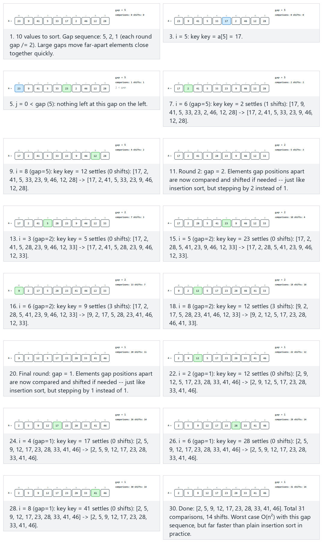
In the picker, also try reverse sorted — large gaps close long distances immediately and compare it against section 4's plain insertion sort on the same reverse-sorted input: watch the comparison and shift counts drop sharply once elements no longer have to cross the whole array one cell at a time. Or press 🎲 for random data, or type your own array.
5.4 Try it
Full program: shell_sort.c / ShellSort.java
/* Week 10 -- Sorting
 * Shell sort: insertion sort, but comparing elements `gap` apart instead of
 * adjacent; the gap starts at n/2 and halves every round down to 1. Prints
 * the array after every gap round and the total comparisons/shifts.
 * CEN207 Data Structures (formerly CE205)
 */
#include <stdio.h>

static void print_array(const int a[], int n) {
    printf("[");
    for (int i = 0; i < n; i++) printf("%d%s", a[i], i + 1 < n ? ", " : "");
    printf("]\n");
}

void shell_sort(int a[], int n, int *comparisons, int *shifts) {
    for (int gap = n / 2; gap > 0; gap /= 2) {
        for (int i = gap; i < n; i++) {
            int key = a[i];
            int j = i;
            while (j >= gap) {
                (*comparisons)++;
                if (a[j - gap] <= key) break;
                a[j] = a[j - gap];
                (*shifts)++;
                j -= gap;
            }
            a[j] = key;
        }
        printf("  gap=%d: ", gap);
        print_array(a, n);
    }
}

static void run_scenario(const char *label, int a[], int n) {
    printf("-- %s --\n", label);
    printf("before: ");
    print_array(a, n);
    int comparisons = 0, shifts = 0;
    shell_sort(a, n, &comparisons, &shifts);
    printf("after:  ");
    print_array(a, n);
    printf("total: %d comparisons, %d shifts\n\n", comparisons, shifts);
}

int main(void) {
    int normal[] = {23, 9, 41, 5, 33, 17, 2, 46, 12, 28};
    int hard[] = {50, 3, 47, 8, 44, 12, 39, 16, 34, 20, 29, 24, 25, 27, 1, 45};
    int already_sorted[] = {1, 2, 3, 4, 5, 6, 7, 8, 9, 10, 11, 12};
    int reverse_sorted[] = {12, 11, 10, 9, 8, 7, 6, 5, 4, 3, 2, 1};

    run_scenario("normal: 10 values, gap sequence 5, 2, 1", normal, 10);
    run_scenario("hard: 16 values, gap sequence 8, 4, 2, 1", hard, 16);
    run_scenario("edge: already sorted -- zero shifts at every gap", already_sorted, 12);
    run_scenario("edge: reverse sorted -- large gaps close long distances immediately", reverse_sorted, 12);

    return 0;
}
/* Week 10 -- Sorting
 * Shell sort: insertion sort, but comparing elements `gap` apart instead of
 * adjacent; the gap starts at n/2 and halves every round down to 1. Prints
 * the array after every gap round and the total comparisons/shifts.
 * CEN207 Data Structures (formerly CE205)
 */
public class ShellSort {
    static int comparisons, shifts;

    static void printArray(int[] a) {
        StringBuilder sb = new StringBuilder("[");
        for (int i = 0; i < a.length; i++) { sb.append(a[i]); if (i + 1 < a.length) sb.append(", "); }
        sb.append(']');
        System.out.println(sb);
    }

    static void shellSort(int[] a) {
        int n = a.length;
        for (int gap = n / 2; gap > 0; gap /= 2) {
            for (int i = gap; i < n; i++) {
                int key = a[i];
                int j = i;
                while (j >= gap) {
                    comparisons++;
                    if (a[j - gap] <= key) break;
                    a[j] = a[j - gap];
                    shifts++;
                    j -= gap;
                }
                a[j] = key;
            }
            System.out.print("  gap=" + gap + ": ");
            printArray(a);
        }
    }

    static void runScenario(String label, int[] a) {
        System.out.println("-- " + label + " --");
        System.out.print("before: ");
        printArray(a);
        comparisons = 0; shifts = 0;
        shellSort(a);
        System.out.print("after:  ");
        printArray(a);
        System.out.println("total: " + comparisons + " comparisons, " + shifts + " shifts");
        System.out.println();
    }

    public static void main(String[] args) {
        int[] normal = {23, 9, 41, 5, 33, 17, 2, 46, 12, 28};
        int[] hard = {50, 3, 47, 8, 44, 12, 39, 16, 34, 20, 29, 24, 25, 27, 1, 45};
        int[] alreadySorted = {1, 2, 3, 4, 5, 6, 7, 8, 9, 10, 11, 12};
        int[] reverseSorted = {12, 11, 10, 9, 8, 7, 6, 5, 4, 3, 2, 1};

        runScenario("normal: 10 values, gap sequence 5, 2, 1", normal);
        runScenario("hard: 16 values, gap sequence 8, 4, 2, 1", hard);
        runScenario("edge: already sorted -- zero shifts at every gap", alreadySorted);
        runScenario("edge: reverse sorted -- large gaps close long distances immediately", reverseSorted);
    }
}
Try it
Expected output:
-- normal: 10 values, gap sequence 5, 2, 1 --
before: [23, 9, 41, 5, 33, 17, 2, 46, 12, 28]
  gap=5: [17, 2, 41, 5, 28, 23, 9, 46, 12, 33]
  gap=2: [9, 2, 12, 5, 17, 23, 28, 33, 41, 46]
  gap=1: [2, 5, 9, 12, 17, 23, 28, 33, 41, 46]
after:  [2, 5, 9, 12, 17, 23, 28, 33, 41, 46]
total: 31 comparisons, 14 shifts

-- hard: 16 values, gap sequence 8, 4, 2, 1 --
before: [50, 3, 47, 8, 44, 12, 39, 16, 34, 20, 29, 24, 25, 27, 1, 45]
  gap=8: [34, 3, 29, 8, 25, 12, 1, 16, 50, 20, 47, 24, 44, 27, 39, 45]
  gap=4: [25, 3, 1, 8, 34, 12, 29, 16, 44, 20, 39, 24, 50, 27, 47, 45]
  gap=2: [1, 3, 25, 8, 29, 12, 34, 16, 39, 20, 44, 24, 47, 27, 50, 45]
  gap=1: [1, 3, 8, 12, 16, 20, 24, 25, 27, 29, 34, 39, 44, 45, 47, 50]
after:  [1, 3, 8, 12, 16, 20, 24, 25, 27, 29, 34, 39, 44, 45, 47, 50]
total: 76 comparisons, 34 shifts

-- edge: already sorted -- zero shifts at every gap --
before: [1, 2, 3, 4, 5, 6, 7, 8, 9, 10, 11, 12]
  gap=6: [1, 2, 3, 4, 5, 6, 7, 8, 9, 10, 11, 12]
  gap=3: [1, 2, 3, 4, 5, 6, 7, 8, 9, 10, 11, 12]
  gap=1: [1, 2, 3, 4, 5, 6, 7, 8, 9, 10, 11, 12]
after:  [1, 2, 3, 4, 5, 6, 7, 8, 9, 10, 11, 12]
total: 26 comparisons, 0 shifts

-- edge: reverse sorted -- large gaps close long distances immediately --
before: [12, 11, 10, 9, 8, 7, 6, 5, 4, 3, 2, 1]
  gap=6: [6, 5, 4, 3, 2, 1, 12, 11, 10, 9, 8, 7]
  gap=3: [3, 2, 1, 6, 5, 4, 9, 8, 7, 12, 11, 10]
  gap=1: [1, 2, 3, 4, 5, 6, 7, 8, 9, 10, 11, 12]
after:  [1, 2, 3, 4, 5, 6, 7, 8, 9, 10, 11, 12]
total: 39 comparisons, 24 shifts
5.5 Complexity, mistakes, self-check
Complexity. Depends on the gap sequence — a famous, still slightly open research question in its own right. With the simple halving sequence used here (n/2, n/4, ..., 1), the worst case is O(n^2) (though in practice, on nearly every real input, it runs far faster than plain insertion sort — compare the reverse-sorted totals above, 39 comparisons for shell sort versus 66 for plain insertion sort on the same 12 values). Better gap sequences exist — Hibbard's (2^k - 1), Sedgewick's, and others — that provably lower the worst case further, to roughly O(n^{4/3}) or better, but they are outside this course's scope; the important idea is the gap itself, not which exact sequence of gaps is optimal. Space: O(1), in place. Shell sort is NOT stable: moving elements by gap > 1 positions at a time can easily swap two equal-keyed elements past each other, exactly like selection sort's long-range swap.
Common mistakes
- Using a fixed, non-shrinking gap, or a gap sequence that does not end at exactly
1. If the final pass is not a plain (gap = 1) insertion sort, the array is not guaranteed to end up fully sorted — only withingapof its correct position. - Off-by-one on the inner loop bound. The condition must be
j >= gap(there must be an elementgappositions to the left to compare against), notj >= 0— the latter would reada[j - gap]with a negative index oncej < gap. - Assuming shell sort is "just insertion sort" and therefore stable. It is not — only the very last pass (
gap = 1) behaves like plain insertion sort; every earlier pass moves elements past others that are more thangapapart in the ORIGINAL array but land in between after earlier passes, which can reorder ties.
Self-check: why does a large first gap help so much?
In the reverse-sorted example above (n = 12), the value 1 starts at the last position and must end at the first. Trace how many total gap-sized jumps it takes to get there across the gap=6, gap=3, and gap=1 passes combined, versus how many single-cell shifts plain insertion sort would need for that same value alone.
Answer. Plain insertion sort would need exactly 11 single-cell shifts to move the value 1 from index 11 to index 0. With shell sort's gap sequence, 1 shifts from index 11 to index 5 during the gap=6 pass (one shift of size 6), then from index 5 to index 2 during the gap=3 pass (one shift of size 3), then from index 2 to index 0 during the final gap=1 pass (two shifts of size 1) — four shifts in total, covering the same eleven-position distance, because the early large-gap passes each cover far more ground per shift.
6. Merge sort
6.1 A question to start
Everything so far has been a variation on "move elements around inside one array." What if, instead, you split the array into two halves, sorted each half completely and independently, and then just combined the two sorted halves? Combining two already-sorted lists is cheap — walk both from the front, always take the smaller of the two current elements — so the only remaining question is how to sort each half. The answer: the same way, recursively, until a half is small enough (one element) to be trivially sorted already. This is divide and conquer, and merge sort is its founding example in computer science, described by John von Neumann in 1945, in one of the very first algorithms ever written for a stored-program computer.
6.2 The idea, and why it guarantees O(n log n)
Split the range [lo, hi) at its midpoint into two halves. Recursively sort each half. Merge the two now-sorted halves back together using an auxiliary array: repeatedly compare the front of each half, copy the smaller one, and advance that half's pointer; once one half runs out, copy the rest of the other half straight across. Because the array is halved at every level of recursion, there are exactly log2(n) levels; because every level's merges together touch every element exactly once, each level costs O(n); total cost: O(n log n), in every case — best, average, and worst — unlike every algorithm you have met so far this week. That "every case" guarantee is merge sort's entire point, and its price is the auxiliary array: merge sort needs O(n) extra memory, unlike the in-place sorts of sections 2–5.
Merge sort comes in two equivalent forms that reach the identical result by different routes, and both get their own animation this week.
6.3 Top-down (recursive): the recursion tree, drawn as rows
The merge-sort animation below draws the recursion literally: each row is one recursion depth. The top rows, going down, show the array being split — d=0 is the whole array; d=1 shows it divided into two halves by a brace; d=2 into four quarters; and so on down to the row where every brace covers a single element. Splitting never changes any value, only the brace boundaries — nothing is copied yet. Then, still going down the same set of rows, the picture flips to merging: the deepest row's single-element "runs" are merged, two at a time, into the row below; those pairs are merged into the row below that; and so on, until the very last row is the complete, sorted array. The first merge in the whole animation is shown one comparison at a time; every later merge is shown as a single before/after step, since the comparison mechanic is identical every time — only the runs being merged get longer.
void merge(int a[], int lo, int mid, int hi, int tmp[]) {
    int i = lo, j = mid, k = lo;
    while (i < mid && j < hi)
        tmp[k++] = (a[i] <= a[j]) ? a[i++] : a[j++];
    while (i < mid) tmp[k++] = a[i++];    /* copy the left leftovers */
    while (j < hi)  tmp[k++] = a[j++];    /* copy the right leftovers */
    for (int x = lo; x < hi; x++) a[x] = tmp[x];
}

void merge_sort(int a[], int lo, int hi, int tmp[]) {
    if (hi - lo <= 1) return;             /* base case: 0 or 1 elements */
    int mid = lo + (hi - lo) / 2;
    merge_sort(a, lo, mid, tmp);          /* sort the left half */
    merge_sort(a, mid, hi, tmp);          /* sort the right half */
    merge(a, lo, mid, hi, tmp);           /* merge the two sorted halves */
}
void merge(int[] a, int lo, int mid, int hi, int[] tmp) {
    int i = lo, j = mid, k = lo;
    while (i < mid && j < hi)
        tmp[k++] = (a[i] <= a[j]) ? a[i++] : a[j++];
    while (i < mid) tmp[k++] = a[i++];    // copy the left leftovers
    while (j < hi)  tmp[k++] = a[j++];    // copy the right leftovers
    for (int x = lo; x < hi; x++) a[x] = tmp[x];
}

void mergeSort(int[] a, int lo, int hi, int[] tmp) {
    if (hi - lo <= 1) return;             // base case: 0 or 1 elements
    int mid = lo + (hi - lo) / 2;
    mergeSort(a, lo, mid, tmp);           // sort the left half
    mergeSort(a, mid, hi, tmp);           // sort the right half
    merge(a, lo, mid, hi, tmp);           // merge the two sorted halves
}
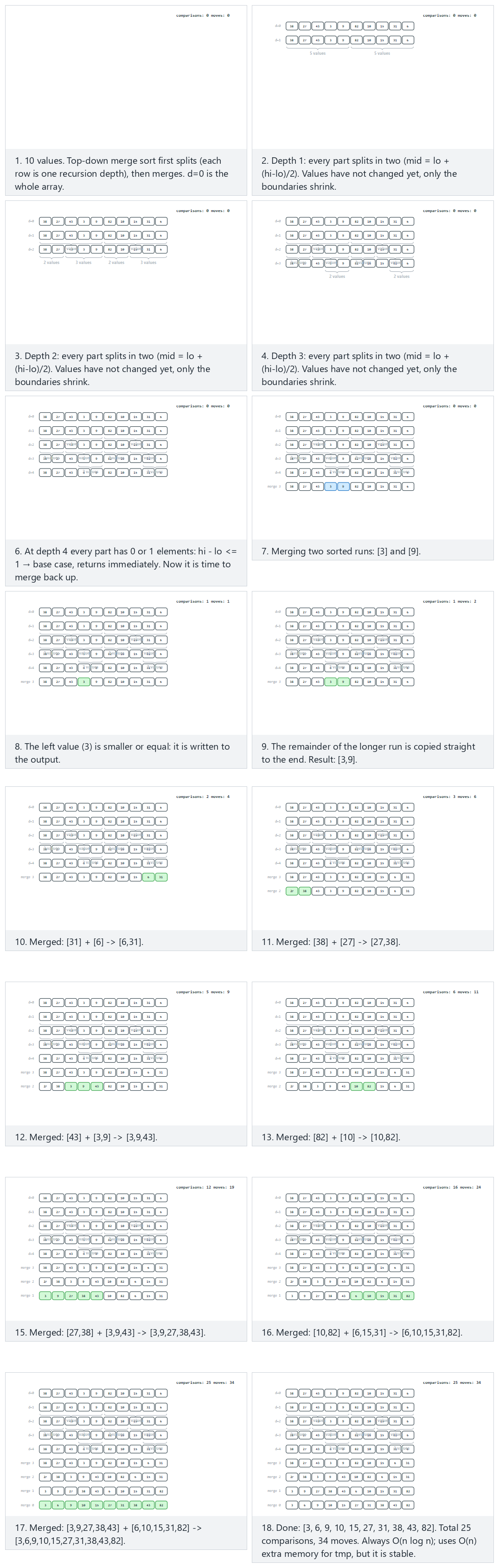
In the picker, also try already sorted — every split and merge still runs (merge sort's guarantee is that it costs O(n log n) regardless of input order — there is no early exit anywhere in this algorithm), or press 🎲 for random data, or type your own array.
Full program: merge_sort.c / MergeSort.java
/* Week 10 -- Sorting
 * Merge sort, top-down (recursive): split the range in half, recursively
 * sort each half, then merge the two sorted halves with an auxiliary
 * array. Prints every merge (its two input runs and the merged result)
 * and the total comparisons/moves.
 * CEN207 Data Structures (formerly CE205)
 */
#include <stdio.h>

static int comparisons, moves;

static void print_range(const int a[], int lo, int hi) {
    printf("[");
    for (int i = lo; i < hi; i++) printf("%d%s", a[i], i + 1 < hi ? "," : "");
    printf("]");
}

void merge(int a[], int lo, int mid, int hi, int tmp[]) {
    int i = lo, j = mid, k = lo;
    while (i < mid && j < hi) {
        comparisons++;
        tmp[k++] = (a[i] <= a[j]) ? a[i++] : a[j++];
        moves++;
    }
    while (i < mid) { tmp[k++] = a[i++]; moves++; }
    while (j < hi) { tmp[k++] = a[j++]; moves++; }
    printf("  merge ");
    print_range(a, lo, mid);
    printf(" + ");
    print_range(a, mid, hi);
    printf(" -> ");
    for (int x = lo; x < hi; x++) a[x] = tmp[x];
    print_range(a, lo, hi);
    printf("\n");
}

void merge_sort(int a[], int lo, int hi, int tmp[]) {
    if (hi - lo <= 1) return;
    int mid = lo + (hi - lo) / 2;
    merge_sort(a, lo, mid, tmp);
    merge_sort(a, mid, hi, tmp);
    merge(a, lo, mid, hi, tmp);
}

static void print_array(const int a[], int n) { print_range(a, 0, n); printf("\n"); }

static void run_scenario(const char *label, int a[], int n) {
    printf("-- %s --\n", label);
    printf("before: ");
    print_array(a, n);
    int tmp[64];
    comparisons = 0; moves = 0;
    merge_sort(a, 0, n, tmp);
    printf("after:  ");
    print_array(a, n);
    printf("total: %d comparisons, %d moves\n\n", comparisons, moves);
}

int main(void) {
    int normal[] = {38, 27, 43, 3, 9, 82, 10, 15, 31, 6};
    int hard[] = {45, 2, 38, 9, 33, 14, 29, 6, 41, 18, 24, 11, 36, 20};
    int already_sorted[] = {1, 2, 3, 4, 5, 6, 7, 8, 9, 10, 11, 12};
    int reverse_sorted[] = {12, 11, 10, 9, 8, 7, 6, 5, 4, 3, 2, 1};

    run_scenario("normal: 10 unordered values", normal, 10);
    run_scenario("hard: 14 values, uneven splits", hard, 14);
    run_scenario("edge: already sorted -- every split and merge still runs", already_sorted, 12);
    run_scenario("edge: reverse sorted", reverse_sorted, 12);

    return 0;
}
/* Week 10 -- Sorting
 * Merge sort, top-down (recursive): split the range in half, recursively
 * sort each half, then merge the two sorted halves with an auxiliary
 * array. Prints every merge (its two input runs and the merged result)
 * and the total comparisons/moves.
 * CEN207 Data Structures (formerly CE205)
 */
public class MergeSort {
    static int comparisons, moves;

    static String rangeStr(int[] a, int lo, int hi) {
        StringBuilder sb = new StringBuilder("[");
        for (int i = lo; i < hi; i++) { sb.append(a[i]); if (i + 1 < hi) sb.append(','); }
        sb.append(']');
        return sb.toString();
    }

    static void merge(int[] a, int lo, int mid, int hi, int[] tmp) {
        int i = lo, j = mid, k = lo;
        String leftBefore = rangeStr(a, lo, mid), rightBefore = rangeStr(a, mid, hi);
        while (i < mid && j < hi) {
            comparisons++;
            tmp[k++] = (a[i] <= a[j]) ? a[i++] : a[j++];
            moves++;
        }
        while (i < mid) { tmp[k++] = a[i++]; moves++; }
        while (j < hi) { tmp[k++] = a[j++]; moves++; }
        for (int x = lo; x < hi; x++) a[x] = tmp[x];
        System.out.println("  merge " + leftBefore + " + " + rightBefore + " -> " + rangeStr(a, lo, hi));
    }

    static void mergeSort(int[] a, int lo, int hi, int[] tmp) {
        if (hi - lo <= 1) return;
        int mid = lo + (hi - lo) / 2;
        mergeSort(a, lo, mid, tmp);
        mergeSort(a, mid, hi, tmp);
        merge(a, lo, mid, hi, tmp);
    }

    static void printArray(int[] a) { System.out.println(rangeStr(a, 0, a.length)); }

    static void runScenario(String label, int[] a) {
        System.out.println("-- " + label + " --");
        System.out.print("before: ");
        printArray(a);
        int[] tmp = new int[a.length];
        comparisons = 0; moves = 0;
        mergeSort(a, 0, a.length, tmp);
        System.out.print("after:  ");
        printArray(a);
        System.out.println("total: " + comparisons + " comparisons, " + moves + " moves");
        System.out.println();
    }

    public static void main(String[] args) {
        int[] normal = {38, 27, 43, 3, 9, 82, 10, 15, 31, 6};
        int[] hard = {45, 2, 38, 9, 33, 14, 29, 6, 41, 18, 24, 11, 36, 20};
        int[] alreadySorted = {1, 2, 3, 4, 5, 6, 7, 8, 9, 10, 11, 12};
        int[] reverseSorted = {12, 11, 10, 9, 8, 7, 6, 5, 4, 3, 2, 1};

        runScenario("normal: 10 unordered values", normal);
        runScenario("hard: 14 values, uneven splits", hard);
        runScenario("edge: already sorted -- every split and merge still runs", alreadySorted);
        runScenario("edge: reverse sorted", reverseSorted);
    }
}
Try it
Expected output:
-- normal: 10 unordered values --
before: [38,27,43,3,9,82,10,15,31,6]
  merge [38] + [27] -> [27,38]
  merge [3] + [9] -> [3,9]
  merge [43] + [3,9] -> [3,9,43]
  merge [27,38] + [3,9,43] -> [3,9,27,38,43]
  merge [82] + [10] -> [10,82]
  merge [31] + [6] -> [6,31]
  merge [15] + [6,31] -> [6,15,31]
  merge [10,82] + [6,15,31] -> [6,10,15,31,82]
  merge [3,9,27,38,43] + [6,10,15,31,82] -> [3,6,9,10,15,27,31,38,43,82]
after:  [3,6,9,10,15,27,31,38,43,82]
total: 25 comparisons, 34 moves

-- hard: 14 values, uneven splits --
before: [45,2,38,9,33,14,29,6,41,18,24,11,36,20]
  merge [2] + [38] -> [2,38]
  merge [45] + [2,38] -> [2,38,45]
  merge [9] + [33] -> [9,33]
  merge [14] + [29] -> [14,29]
  merge [9,33] + [14,29] -> [9,14,29,33]
  merge [2,38,45] + [9,14,29,33] -> [2,9,14,29,33,38,45]
  merge [41] + [18] -> [18,41]
  merge [6] + [18,41] -> [6,18,41]
  merge [24] + [11] -> [11,24]
  merge [36] + [20] -> [20,36]
  merge [11,24] + [20,36] -> [11,20,24,36]
  merge [6,18,41] + [11,20,24,36] -> [6,11,18,20,24,36,41]
  merge [2,9,14,29,33,38,45] + [6,11,18,20,24,36,41] -> [2,6,9,11,14,18,20,24,29,33,36,38,41,45]
after:  [2,6,9,11,14,18,20,24,29,33,36,38,41,45]
total: 39 comparisons, 54 moves

-- edge: already sorted -- every split and merge still runs --
before: [1,2,3,4,5,6,7,8,9,10,11,12]
  merge [2] + [3] -> [2,3]
  merge [1] + [2,3] -> [1,2,3]
  merge [5] + [6] -> [5,6]
  merge [4] + [5,6] -> [4,5,6]
  merge [1,2,3] + [4,5,6] -> [1,2,3,4,5,6]
  merge [8] + [9] -> [8,9]
  merge [7] + [8,9] -> [7,8,9]
  merge [11] + [12] -> [11,12]
  merge [10] + [11,12] -> [10,11,12]
  merge [7,8,9] + [10,11,12] -> [7,8,9,10,11,12]
  merge [1,2,3,4,5,6] + [7,8,9,10,11,12] -> [1,2,3,4,5,6,7,8,9,10,11,12]
after:  [1,2,3,4,5,6,7,8,9,10,11,12]
total: 20 comparisons, 44 moves

-- edge: reverse sorted --
before: [12,11,10,9,8,7,6,5,4,3,2,1]
  merge [11] + [10] -> [10,11]
  merge [12] + [10,11] -> [10,11,12]
  merge [8] + [7] -> [7,8]
  merge [9] + [7,8] -> [7,8,9]
  merge [10,11,12] + [7,8,9] -> [7,8,9,10,11,12]
  merge [5] + [4] -> [4,5]
  merge [6] + [4,5] -> [4,5,6]
  merge [2] + [1] -> [1,2]
  merge [3] + [1,2] -> [1,2,3]
  merge [4,5,6] + [1,2,3] -> [1,2,3,4,5,6]
  merge [7,8,9,10,11,12] + [1,2,3,4,5,6] -> [1,2,3,4,5,6,7,8,9,10,11,12]
after:  [1,2,3,4,5,6,7,8,9,10,11,12]
total: 24 comparisons, 44 moves
6.4 Bottom-up (iterative): no recursion at all
merge-sort-bottom-up reaches the identical result with no recursive calls whatsoever. Treat every single element as a sorted run of width 1 (trivially true). Merge adjacent runs, left to right across the whole array, into runs of width 2. Merge those into runs of width 4. Keep doubling the run width until one round produces a single run covering the whole array — the array is sorted, in exactly log2(n) rounds, using the same merge() helper as the top-down version, just reached by an explicit loop over widths instead of a call stack.
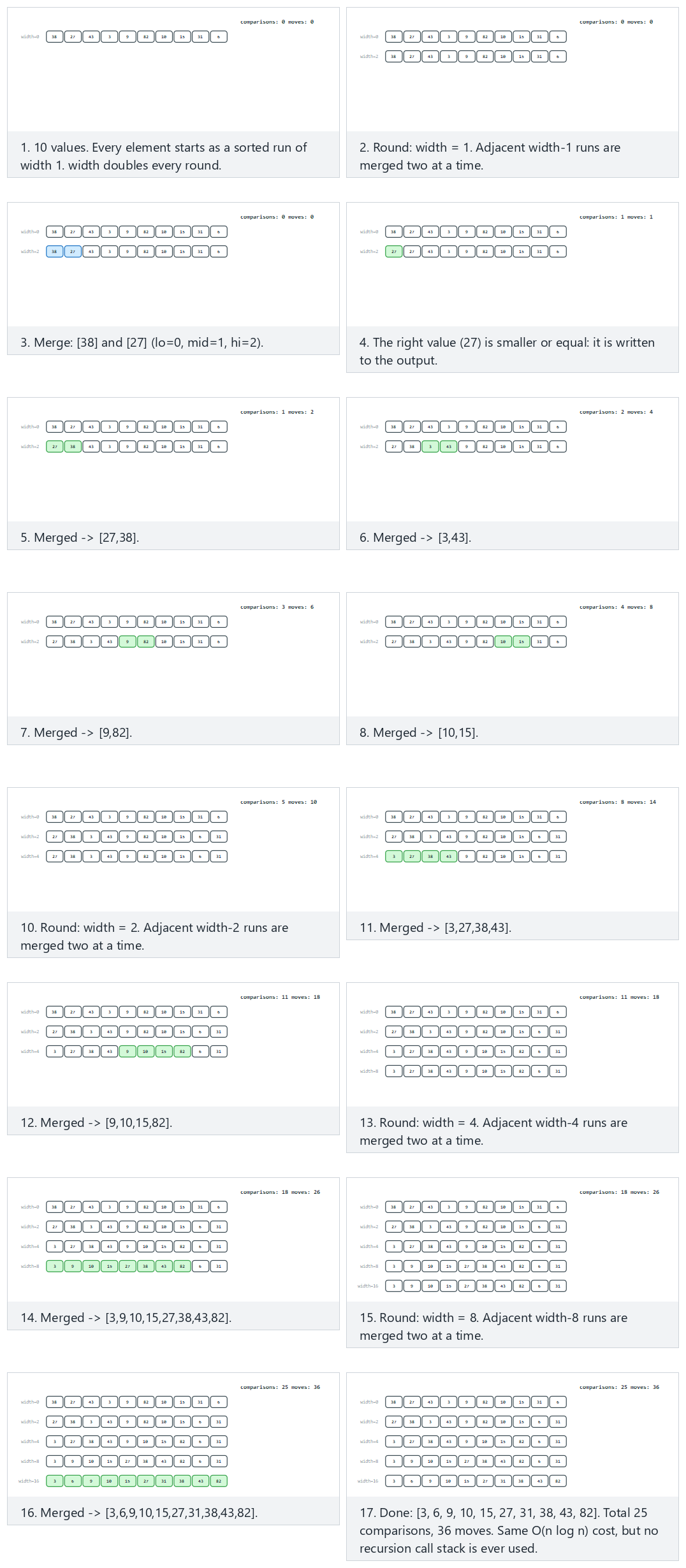
In the picker, also try 16 values: n is exactly a power of 2, every round is even versus the hard example (14 values, so the last round of each width has an uneven, partial pair) — notice the algorithm handles both without any special-casing, thanks to the Math.min / ternary clamp on hi. Or press 🎲 for random data, or type your own array.
Full program: merge_sort_bottom_up.c / MergeSortBottomUp.java
/* Week 10 -- Sorting
 * Merge sort, bottom-up (iterative): no recursion. Treat every element as
 * a sorted run of width 1, merge adjacent runs into width-2 runs, then
 * width-4, doubling every round until one run covers the whole array.
 * Prints every merge and the total comparisons/moves.
 * CEN207 Data Structures (formerly CE205)
 */
#include <stdio.h>

static int comparisons, moves;

static void print_range(const int a[], int lo, int hi) {
    printf("[");
    for (int i = lo; i < hi; i++) printf("%d%s", a[i], i + 1 < hi ? "," : "");
    printf("]");
}

static void merge(int a[], int lo, int mid, int hi, int tmp[]) {
    int i = lo, j = mid, k = lo;
    printf("  merge ");
    print_range(a, lo, mid);
    printf(" + ");
    print_range(a, mid, hi);
    while (i < mid && j < hi) {
        comparisons++;
        tmp[k++] = (a[i] <= a[j]) ? a[i++] : a[j++];
        moves++;
    }
    while (i < mid) { tmp[k++] = a[i++]; moves++; }
    while (j < hi) { tmp[k++] = a[j++]; moves++; }
    for (int x = lo; x < hi; x++) a[x] = tmp[x];
    printf(" -> ");
    print_range(a, lo, hi);
    printf("\n");
}

void merge_sort_bottom_up(int a[], int n, int tmp[]) {
    for (int width = 1; width < n; width *= 2) {
        printf(" width=%d:\n", width);
        for (int lo = 0; lo < n - width; lo += 2 * width) {
            int mid = lo + width;
            int hi = mid + width < n ? mid + width : n;
            merge(a, lo, mid, hi, tmp);
        }
    }
}

static void print_array(const int a[], int n) { print_range(a, 0, n); printf("\n"); }

static void run_scenario(const char *label, int a[], int n) {
    printf("-- %s --\n", label);
    printf("before: ");
    print_array(a, n);
    int tmp[64];
    comparisons = 0; moves = 0;
    merge_sort_bottom_up(a, n, tmp);
    printf("after:  ");
    print_array(a, n);
    printf("total: %d comparisons, %d moves\n\n", comparisons, moves);
}

int main(void) {
    int normal[] = {38, 27, 43, 3, 9, 82, 10, 15, 31, 6};
    int power_of_two[] = {16, 3, 9, 14, 1, 12, 7, 10, 5, 15, 2, 11, 8, 13, 4, 6};
    int already_sorted[] = {1, 2, 3, 4, 5, 6, 7, 8, 9, 10, 11, 12};
    int reverse_sorted[] = {12, 11, 10, 9, 8, 7, 6, 5, 4, 3, 2, 1};

    run_scenario("normal: 10 unordered values", normal, 10);
    run_scenario("hard: 16 values, n is exactly a power of 2", power_of_two, 16);
    run_scenario("edge: already sorted -- every round still runs", already_sorted, 12);
    run_scenario("edge: reverse sorted", reverse_sorted, 12);

    return 0;
}
/* Week 10 -- Sorting
 * Merge sort, bottom-up (iterative): no recursion. Treat every element as
 * a sorted run of width 1, merge adjacent runs into width-2 runs, then
 * width-4, doubling every round until one run covers the whole array.
 * Prints every merge and the total comparisons/moves.
 * CEN207 Data Structures (formerly CE205)
 */
public class MergeSortBottomUp {
    static int comparisons, moves;

    static String rangeStr(int[] a, int lo, int hi) {
        StringBuilder sb = new StringBuilder("[");
        for (int i = lo; i < hi; i++) { sb.append(a[i]); if (i + 1 < hi) sb.append(','); }
        sb.append(']');
        return sb.toString();
    }

    static void merge(int[] a, int lo, int mid, int hi, int[] tmp) {
        int i = lo, j = mid, k = lo;
        String leftBefore = rangeStr(a, lo, mid), rightBefore = rangeStr(a, mid, hi);
        while (i < mid && j < hi) {
            comparisons++;
            tmp[k++] = (a[i] <= a[j]) ? a[i++] : a[j++];
            moves++;
        }
        while (i < mid) { tmp[k++] = a[i++]; moves++; }
        while (j < hi) { tmp[k++] = a[j++]; moves++; }
        for (int x = lo; x < hi; x++) a[x] = tmp[x];
        System.out.println("  merge " + leftBefore + " + " + rightBefore + " -> " + rangeStr(a, lo, hi));
    }

    static void mergeSortBottomUp(int[] a, int n, int[] tmp) {
        for (int width = 1; width < n; width *= 2) {
            System.out.println(" width=" + width + ":");
            for (int lo = 0; lo < n - width; lo += 2 * width) {
                int mid = lo + width;
                int hi = Math.min(mid + width, n);
                merge(a, lo, mid, hi, tmp);
            }
        }
    }

    static void printArray(int[] a) { System.out.println(rangeStr(a, 0, a.length)); }

    static void runScenario(String label, int[] a) {
        System.out.println("-- " + label + " --");
        System.out.print("before: ");
        printArray(a);
        int[] tmp = new int[a.length];
        comparisons = 0; moves = 0;
        mergeSortBottomUp(a, a.length, tmp);
        System.out.print("after:  ");
        printArray(a);
        System.out.println("total: " + comparisons + " comparisons, " + moves + " moves");
        System.out.println();
    }

    public static void main(String[] args) {
        int[] normal = {38, 27, 43, 3, 9, 82, 10, 15, 31, 6};
        int[] powerOfTwo = {16, 3, 9, 14, 1, 12, 7, 10, 5, 15, 2, 11, 8, 13, 4, 6};
        int[] alreadySorted = {1, 2, 3, 4, 5, 6, 7, 8, 9, 10, 11, 12};
        int[] reverseSorted = {12, 11, 10, 9, 8, 7, 6, 5, 4, 3, 2, 1};

        runScenario("normal: 10 unordered values", normal);
        runScenario("hard: 16 values, n is exactly a power of 2", powerOfTwo);
        runScenario("edge: already sorted -- every round still runs", alreadySorted);
        runScenario("edge: reverse sorted", reverseSorted);
    }
}
Try it
Expected output:
-- normal: 10 unordered values --
before: [38,27,43,3,9,82,10,15,31,6]
 width=1:
  merge [38] + [27] -> [27,38]
  merge [43] + [3] -> [3,43]
  merge [9] + [82] -> [9,82]
  merge [10] + [15] -> [10,15]
  merge [31] + [6] -> [6,31]
 width=2:
  merge [27,38] + [3,43] -> [3,27,38,43]
  merge [9,82] + [10,15] -> [9,10,15,82]
 width=4:
  merge [3,27,38,43] + [9,10,15,82] -> [3,9,10,15,27,38,43,82]
 width=8:
  merge [3,9,10,15,27,38,43,82] + [6,31] -> [3,6,9,10,15,27,31,38,43,82]
after:  [3,6,9,10,15,27,31,38,43,82]
total: 25 comparisons, 36 moves

-- hard: 16 values, n is exactly a power of 2 --
before: [16,3,9,14,1,12,7,10,5,15,2,11,8,13,4,6]
 width=1:
  merge [16] + [3] -> [3,16]
  merge [9] + [14] -> [9,14]
  merge [1] + [12] -> [1,12]
  merge [7] + [10] -> [7,10]
  merge [5] + [15] -> [5,15]
  merge [2] + [11] -> [2,11]
  merge [8] + [13] -> [8,13]
  merge [4] + [6] -> [4,6]
 width=2:
  merge [3,16] + [9,14] -> [3,9,14,16]
  merge [1,12] + [7,10] -> [1,7,10,12]
  merge [5,15] + [2,11] -> [2,5,11,15]
  merge [8,13] + [4,6] -> [4,6,8,13]
 width=4:
  merge [3,9,14,16] + [1,7,10,12] -> [1,3,7,9,10,12,14,16]
  merge [2,5,11,15] + [4,6,8,13] -> [2,4,5,6,8,11,13,15]
 width=8:
  merge [1,3,7,9,10,12,14,16] + [2,4,5,6,8,11,13,15] -> [1,2,3,4,5,6,7,8,9,10,11,12,13,14,15,16]
after:  [1,2,3,4,5,6,7,8,9,10,11,12,13,14,15,16]
total: 47 comparisons, 64 moves

-- edge: already sorted -- every round still runs --
before: [1,2,3,4,5,6,7,8,9,10,11,12]
 width=1:
  merge [1] + [2] -> [1,2]
  merge [3] + [4] -> [3,4]
  merge [5] + [6] -> [5,6]
  merge [7] + [8] -> [7,8]
  merge [9] + [10] -> [9,10]
  merge [11] + [12] -> [11,12]
 width=2:
  merge [1,2] + [3,4] -> [1,2,3,4]
  merge [5,6] + [7,8] -> [5,6,7,8]
  merge [9,10] + [11,12] -> [9,10,11,12]
 width=4:
  merge [1,2,3,4] + [5,6,7,8] -> [1,2,3,4,5,6,7,8]
 width=8:
  merge [1,2,3,4,5,6,7,8] + [9,10,11,12] -> [1,2,3,4,5,6,7,8,9,10,11,12]
after:  [1,2,3,4,5,6,7,8,9,10,11,12]
total: 24 comparisons, 44 moves

-- edge: reverse sorted --
before: [12,11,10,9,8,7,6,5,4,3,2,1]
 width=1:
  merge [12] + [11] -> [11,12]
  merge [10] + [9] -> [9,10]
  merge [8] + [7] -> [7,8]
  merge [6] + [5] -> [5,6]
  merge [4] + [3] -> [3,4]
  merge [2] + [1] -> [1,2]
 width=2:
  merge [11,12] + [9,10] -> [9,10,11,12]
  merge [7,8] + [5,6] -> [5,6,7,8]
  merge [3,4] + [1,2] -> [1,2,3,4]
 width=4:
  merge [9,10,11,12] + [5,6,7,8] -> [5,6,7,8,9,10,11,12]
 width=8:
  merge [5,6,7,8,9,10,11,12] + [1,2,3,4] -> [1,2,3,4,5,6,7,8,9,10,11,12]
after:  [1,2,3,4,5,6,7,8,9,10,11,12]
total: 20 comparisons, 44 moves
6.5 Complexity, mistakes, self-check
Complexity. O(n log n) in the best, average, and worst case — the only algorithm this week with that guarantee (heap sort, from Week 4, shares it). Space: O(n) extra, for the tmp array — the price of that guarantee. Merge sort is stable: the merge step's tie-break, a[i] <= a[j], always prefers the LEFT run when the two front elements are equal, and the left run's elements were, by construction, positioned no later than the right run's in the original array — so equal keys keep their relative order all the way up the recursion.
Common mistakes
- Using
<instead of<=in the merge's tie-break.a[i] < a[j]would, on a tie, take from the RIGHT run first — the merge is still numerically correct, but stability is lost. Always use<=(prefer the left run) for a stable ascending merge. - Allocating a fresh
tmparray inside every recursive call, instead of one array of sizenallocated once and reused. It still works, but it turnsO(n)total extra memory intoO(n log n)worth of allocations across the recursion — wasteful and, in a language with manual memory management, a leak risk if any exit path forgets to free it. - Getting
midwrong under overflow, classically writingmid = (lo + hi) / 2instead ofmid = lo + (hi - lo) / 2. For array sizes this course ever uses this makes no observable difference, but the second form is the one that remains correct even for arrays so large thatlo + hiwould overflow a 32-bitint— a habit worth having from the start.
Self-check: top-down versus bottom-up
Both merge_sort and merge_sort_bottom_up produce identical output on identical input and do the same total work. Explain, in one sentence, the one concrete practical advantage bottom-up merge sort has over top-down, and name one advantage top-down has in return.
Answer. Bottom-up merge sort never uses the call stack, so it cannot overflow it no matter how large n is, and it can be written with no recursion in languages or environments where recursion is expensive or disallowed. Top-down merge sort's advantage is that its recursive structure maps directly onto the "divide into independent sub-problems" idea, which makes it easier to adapt — for instance, to stop recursing early and switch to insertion sort once a sub-array is small (a real optimization used by production sort implementations), something that is far more natural to express recursively than as an explicit width-doubling loop.
7. Quick sort
7.1 A question to start
Merge sort guarantees O(n log n) but pays for it with O(n) extra memory. Is there a divide-and-conquer sort that guarantees O(n log n) on average and sorts in place, with no auxiliary array? Tony Hoare invented one in 1959–1960, while a 26-year-old visiting researcher at Moscow State University working on a machine translation project, and published it as "Quicksort" in The Computer Journal in 1962. It remains, to this day, one of the most widely used general-purpose sorting algorithms in real software — including, in various tuned forms, the default array sort in many language standard libraries.
7.2 The idea: partition around a pivot, then recurse
Pick one element of the range as the pivot. Partition the range so that every element <= pivot ends up to its left and every element >= pivot ends up to its right (the pivot itself lands somewhere in between — exactly where depends on which partitioning scheme you use, section 7.3 vs. 7.4). Recursively quick-sort the left part and the right part. Unlike merge sort, there is no separate "combine" step — once partitioning is done and both sides are recursively sorted, the whole range is sorted, because every element on the left is already <= every element on the right. This section covers the two classic partitioning schemes side by side, since they differ in a way that trips up almost everyone the first time.
7.3 Lomuto partitioning: pivot = the last element
Lomuto's scheme (named for Nico Lomuto, who popularized this simpler variant) always picks the range's last element as the pivot. It scans left to right with an index j, maintaining a second index i that marks the right boundary of the "confirmed <= pivot" region built so far: whenever a[j] <= pivot, i advances and a[i] swaps with a[j]. Once the scan finishes, the pivot swaps from the end into position i + 1 — its final, correctly sorted position, guaranteed.
int partition_lomuto(int a[], int lo, int hi) {
    int pivot = a[hi];              /* pivot = last element of the range */
    int i = lo - 1;                 /* boundary of the "<= pivot" region */
    for (int j = lo; j < hi; j++) {
        if (a[j] <= pivot) {
            i++;
            int tmp = a[i]; a[i] = a[j]; a[j] = tmp;
        }
    }
    int tmp2 = a[i + 1]; a[i + 1] = a[hi]; a[hi] = tmp2;   /* pivot to its final spot */
    return i + 1;
}

void quick_sort_lomuto(int a[], int lo, int hi) {
    if (lo < hi) {
        int p = partition_lomuto(a, lo, hi);
        quick_sort_lomuto(a, lo, p - 1);      /* left of the pivot */
        quick_sort_lomuto(a, p + 1, hi);      /* right of the pivot */
    }
}
int partitionLomuto(int[] a, int lo, int hi) {
    int pivot = a[hi];              // pivot = last element of the range
    int i = lo - 1;                 // boundary of the "<= pivot" region
    for (int j = lo; j < hi; j++) {
        if (a[j] <= pivot) {
            i++;
            int tmp = a[i]; a[i] = a[j]; a[j] = tmp;
        }
    }
    int tmp2 = a[i + 1]; a[i + 1] = a[hi]; a[hi] = tmp2;   // pivot to its final spot
    return i + 1;
}

void quickSortLomuto(int[] a, int lo, int hi) {
    if (lo < hi) {
        int p = partitionLomuto(a, lo, hi);
        quickSortLomuto(a, lo, p - 1);        // left of the pivot
        quickSortLomuto(a, p + 1, hi);        // right of the pivot
    }
}
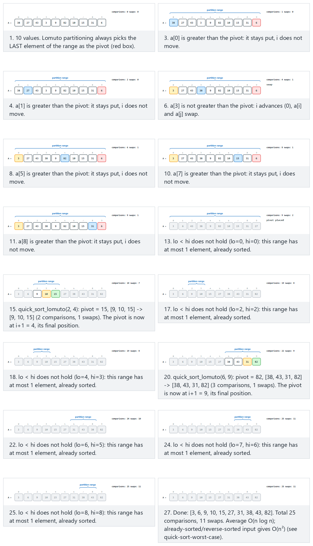
In the picker, also try all equal — every value equals the pivot (watch every comparison still run, but every value sits <= pivot, so i advances every single step) or press 🎲 for random data, or type your own array.
Full program: quick_sort_lomuto.c / QuickSortLomuto.java
/* Week 10 -- Sorting
 * Quick sort with Lomuto partitioning: pivot = last element of the range.
 * `i` marks the boundary of the "<= pivot" region; `j` scans left to
 * right. The pivot then swaps into its final position i+1. Prints every
 * partition call and the total comparisons/swaps.
 * CEN207 Data Structures (formerly CE205)
 */
#include <stdio.h>

static int comparisons, swaps;

static void print_range(const int a[], int lo, int hi) {
    printf("[");
    for (int i = lo; i <= hi; i++) printf("%d%s", a[i], i < hi ? "," : "");
    printf("]");
}

int partition_lomuto(int a[], int lo, int hi) {
    int pivot = a[hi];
    int i = lo - 1;
    for (int j = lo; j < hi; j++) {
        comparisons++;
        if (a[j] <= pivot) {
            i++;
            int tmp = a[i]; a[i] = a[j]; a[j] = tmp;
            if (i != j) swaps++;
        }
    }
    int tmp2 = a[i + 1]; a[i + 1] = a[hi]; a[hi] = tmp2;
    swaps++;
    return i + 1;
}

void quick_sort_lomuto(int a[], int lo, int hi) {
    if (lo < hi) {
        printf("  partition [%d..%d] ", lo, hi);
        print_range(a, lo, hi);
        printf(" pivot=%d -> ", a[hi]);
        int p = partition_lomuto(a, lo, hi);
        print_range(a, lo, hi);
        printf(" (pivot lands at %d)\n", p);
        quick_sort_lomuto(a, lo, p - 1);
        quick_sort_lomuto(a, p + 1, hi);
    }
}

static void print_array(const int a[], int n) { print_range(a, 0, n - 1); printf("\n"); }

static void run_scenario(const char *label, int a[], int n) {
    printf("-- %s --\n", label);
    printf("before: ");
    print_array(a, n);
    comparisons = 0; swaps = 0;
    quick_sort_lomuto(a, 0, n - 1);
    printf("after:  ");
    print_array(a, n);
    printf("total: %d comparisons, %d swaps\n\n", comparisons, swaps);
}

int main(void) {
    int normal[] = {38, 27, 43, 3, 9, 82, 10, 15, 31, 6};
    int repeated[] = {7, 2, 7, 9, 2, 7, 4, 9, 2, 4, 7, 9};
    int already_sorted[] = {1, 2, 3, 4, 5, 6, 7, 8, 9, 10};
    int reverse_sorted[] = {10, 9, 8, 7, 6, 5, 4, 3, 2, 1};

    run_scenario("normal: 10 unordered values", normal, 10);
    run_scenario("hard: 12 values with repeated keys", repeated, 12);
    run_scenario("edge: already sorted -- worst case, every partition is n-1/0", already_sorted, 10);
    run_scenario("edge: reverse sorted -- worst case again", reverse_sorted, 10);

    return 0;
}
/* Week 10 -- Sorting
 * Quick sort with Lomuto partitioning: pivot = last element of the range.
 * `i` marks the boundary of the "<= pivot" region; `j` scans left to
 * right. The pivot then swaps into its final position i+1. Prints every
 * partition call and the total comparisons/swaps.
 * CEN207 Data Structures (formerly CE205)
 */
public class QuickSortLomuto {
    static int comparisons, swaps;

    static String rangeStr(int[] a, int lo, int hi) {
        StringBuilder sb = new StringBuilder("[");
        for (int i = lo; i <= hi; i++) { sb.append(a[i]); if (i < hi) sb.append(','); }
        sb.append(']');
        return sb.toString();
    }

    static int partitionLomuto(int[] a, int lo, int hi) {
        int pivot = a[hi];
        int i = lo - 1;
        for (int j = lo; j < hi; j++) {
            comparisons++;
            if (a[j] <= pivot) {
                i++;
                int tmp = a[i]; a[i] = a[j]; a[j] = tmp;
                if (i != j) swaps++;
            }
        }
        int tmp2 = a[i + 1]; a[i + 1] = a[hi]; a[hi] = tmp2;
        swaps++;
        return i + 1;
    }

    static void quickSortLomuto(int[] a, int lo, int hi) {
        if (lo < hi) {
            String before = rangeStr(a, lo, hi);
            int pivotVal = a[hi];
            int p = partitionLomuto(a, lo, hi);
            System.out.println("  partition [" + lo + ".." + hi + "] " + before + " pivot=" + pivotVal + " -> " + rangeStr(a, lo, hi) + " (pivot lands at " + p + ")");
            quickSortLomuto(a, lo, p - 1);
            quickSortLomuto(a, p + 1, hi);
        }
    }

    static void printArray(int[] a) { System.out.println(rangeStr(a, 0, a.length - 1)); }

    static void runScenario(String label, int[] a) {
        System.out.println("-- " + label + " --");
        System.out.print("before: ");
        printArray(a);
        comparisons = 0; swaps = 0;
        quickSortLomuto(a, 0, a.length - 1);
        System.out.print("after:  ");
        printArray(a);
        System.out.println("total: " + comparisons + " comparisons, " + swaps + " swaps");
        System.out.println();
    }

    public static void main(String[] args) {
        int[] normal = {38, 27, 43, 3, 9, 82, 10, 15, 31, 6};
        int[] repeated = {7, 2, 7, 9, 2, 7, 4, 9, 2, 4, 7, 9};
        int[] alreadySorted = {1, 2, 3, 4, 5, 6, 7, 8, 9, 10};
        int[] reverseSorted = {10, 9, 8, 7, 6, 5, 4, 3, 2, 1};

        runScenario("normal: 10 unordered values", normal);
        runScenario("hard: 12 values with repeated keys", repeated);
        runScenario("edge: already sorted -- worst case, every partition is n-1/0", alreadySorted);
        runScenario("edge: reverse sorted -- worst case again", reverseSorted);
    }
}
Try it
Expected output:
-- normal: 10 unordered values --
before: [38,27,43,3,9,82,10,15,31,6]
  partition [0..9] [38,27,43,3,9,82,10,15,31,6] pivot=6 -> [3,6,43,38,9,82,10,15,31,27] (pivot lands at 1)
  partition [2..9] [43,38,9,82,10,15,31,27] pivot=27 -> [9,10,15,27,38,43,31,82] (pivot lands at 5)
  partition [2..4] [9,10,15] pivot=15 -> [9,10,15] (pivot lands at 4)
  partition [2..3] [9,10] pivot=10 -> [9,10] (pivot lands at 3)
  partition [6..9] [38,43,31,82] pivot=82 -> [38,43,31,82] (pivot lands at 9)
  partition [6..8] [38,43,31] pivot=31 -> [31,43,38] (pivot lands at 6)
  partition [7..8] [43,38] pivot=38 -> [38,43] (pivot lands at 7)
after:  [3,6,9,10,15,27,31,38,43,82]
total: 25 comparisons, 11 swaps

-- hard: 12 values with repeated keys --
before: [7,2,7,9,2,7,4,9,2,4,7,9]
  partition [0..11] [7,2,7,9,2,7,4,9,2,4,7,9] pivot=9 -> [7,2,7,9,2,7,4,9,2,4,7,9] (pivot lands at 11)
  partition [0..10] [7,2,7,9,2,7,4,9,2,4,7] pivot=7 -> [7,2,7,2,7,4,2,4,7,9,9] (pivot lands at 8)
  partition [0..7] [7,2,7,2,7,4,2,4] pivot=4 -> [2,2,4,2,4,7,7,7] (pivot lands at 4)
  partition [0..3] [2,2,4,2] pivot=2 -> [2,2,2,4] (pivot lands at 2)
  partition [0..1] [2,2] pivot=2 -> [2,2] (pivot lands at 1)
  partition [5..7] [7,7,7] pivot=7 -> [7,7,7] (pivot lands at 7)
  partition [5..6] [7,7] pivot=7 -> [7,7] (pivot lands at 6)
  partition [9..10] [9,9] pivot=9 -> [9,9] (pivot lands at 10)
after:  [2,2,2,4,4,7,7,7,7,9,9,9]
total: 36 comparisons, 17 swaps

-- edge: already sorted -- worst case, every partition is n-1/0 --
before: [1,2,3,4,5,6,7,8,9,10]
  partition [0..9] [1,2,3,4,5,6,7,8,9,10] pivot=10 -> [1,2,3,4,5,6,7,8,9,10] (pivot lands at 9)
  partition [0..8] [1,2,3,4,5,6,7,8,9] pivot=9 -> [1,2,3,4,5,6,7,8,9] (pivot lands at 8)
  partition [0..7] [1,2,3,4,5,6,7,8] pivot=8 -> [1,2,3,4,5,6,7,8] (pivot lands at 7)
  partition [0..6] [1,2,3,4,5,6,7] pivot=7 -> [1,2,3,4,5,6,7] (pivot lands at 6)
  partition [0..5] [1,2,3,4,5,6] pivot=6 -> [1,2,3,4,5,6] (pivot lands at 5)
  partition [0..4] [1,2,3,4,5] pivot=5 -> [1,2,3,4,5] (pivot lands at 4)
  partition [0..3] [1,2,3,4] pivot=4 -> [1,2,3,4] (pivot lands at 3)
  partition [0..2] [1,2,3] pivot=3 -> [1,2,3] (pivot lands at 2)
  partition [0..1] [1,2] pivot=2 -> [1,2] (pivot lands at 1)
after:  [1,2,3,4,5,6,7,8,9,10]
total: 45 comparisons, 9 swaps

-- edge: reverse sorted -- worst case again --
before: [10,9,8,7,6,5,4,3,2,1]
  partition [0..9] [10,9,8,7,6,5,4,3,2,1] pivot=1 -> [1,9,8,7,6,5,4,3,2,10] (pivot lands at 0)
  partition [1..9] [9,8,7,6,5,4,3,2,10] pivot=10 -> [9,8,7,6,5,4,3,2,10] (pivot lands at 9)
  partition [1..8] [9,8,7,6,5,4,3,2] pivot=2 -> [2,8,7,6,5,4,3,9] (pivot lands at 1)
  partition [2..8] [8,7,6,5,4,3,9] pivot=9 -> [8,7,6,5,4,3,9] (pivot lands at 8)
  partition [2..7] [8,7,6,5,4,3] pivot=3 -> [3,7,6,5,4,8] (pivot lands at 2)
  partition [3..7] [7,6,5,4,8] pivot=8 -> [7,6,5,4,8] (pivot lands at 7)
  partition [3..6] [7,6,5,4] pivot=4 -> [4,6,5,7] (pivot lands at 3)
  partition [4..6] [6,5,7] pivot=7 -> [6,5,7] (pivot lands at 6)
  partition [4..5] [6,5] pivot=5 -> [5,6] (pivot lands at 4)
after:  [1,2,3,4,5,6,7,8,9,10]
total: 45 comparisons, 9 swaps
7.4 Hoare partitioning: pivot = the first element, two scans
Hoare's original scheme (the one Hoare himself published) picks the first element of the range as the pivot and uses two pointers, i starting just left of the range and j starting just right of it, that scan inward from both ends: i moves right until it finds an element >= pivot; j moves left until it finds an element <= pivot; if the pointers have not yet crossed (i < j), those two elements swap, and scanning continues; once they cross, the partition is done and j is returned. The pivot is not guaranteed to end up at index j — Hoare's partition only guarantees that every element at or before j is <= pivot and every element after j is >= pivot, not that the pivot itself sits exactly at j. That has a direct, easy-to-get -wrong consequence for the recursive calls: they must be (lo, p) and (p + 1, hi) — using p, not p - 1, unlike Lomuto's scheme.
int partition_hoare(int a[], int lo, int hi) {
    int pivot = a[lo];               /* pivot = FIRST element */
    int i = lo - 1, j = hi + 1;
    while (1) {
        do { i++; } while (a[i] < pivot);
        do { j--; } while (a[j] > pivot);
        if (i >= j) return j;
        int tmp = a[i]; a[i] = a[j]; a[j] = tmp;
    }
}

void quick_sort_hoare(int a[], int lo, int hi) {
    if (lo < hi) {
        int p = partition_hoare(a, lo, hi);
        quick_sort_hoare(a, lo, p);       /* note: p, NOT p - 1 */
        quick_sort_hoare(a, p + 1, hi);
    }
}
int partitionHoare(int[] a, int lo, int hi) {
    int pivot = a[lo];               // pivot = FIRST element
    int i = lo - 1, j = hi + 1;
    while (true) {
        do { i++; } while (a[i] < pivot);
        do { j--; } while (a[j] > pivot);
        if (i >= j) return j;
        int tmp = a[i]; a[i] = a[j]; a[j] = tmp;
    }
}

void quickSortHoare(int[] a, int lo, int hi) {
    if (lo < hi) {
        int p = partitionHoare(a, lo, hi);
        quickSortHoare(a, lo, p);         // note: p, NOT p - 1
        quickSortHoare(a, p + 1, hi);
    }
}
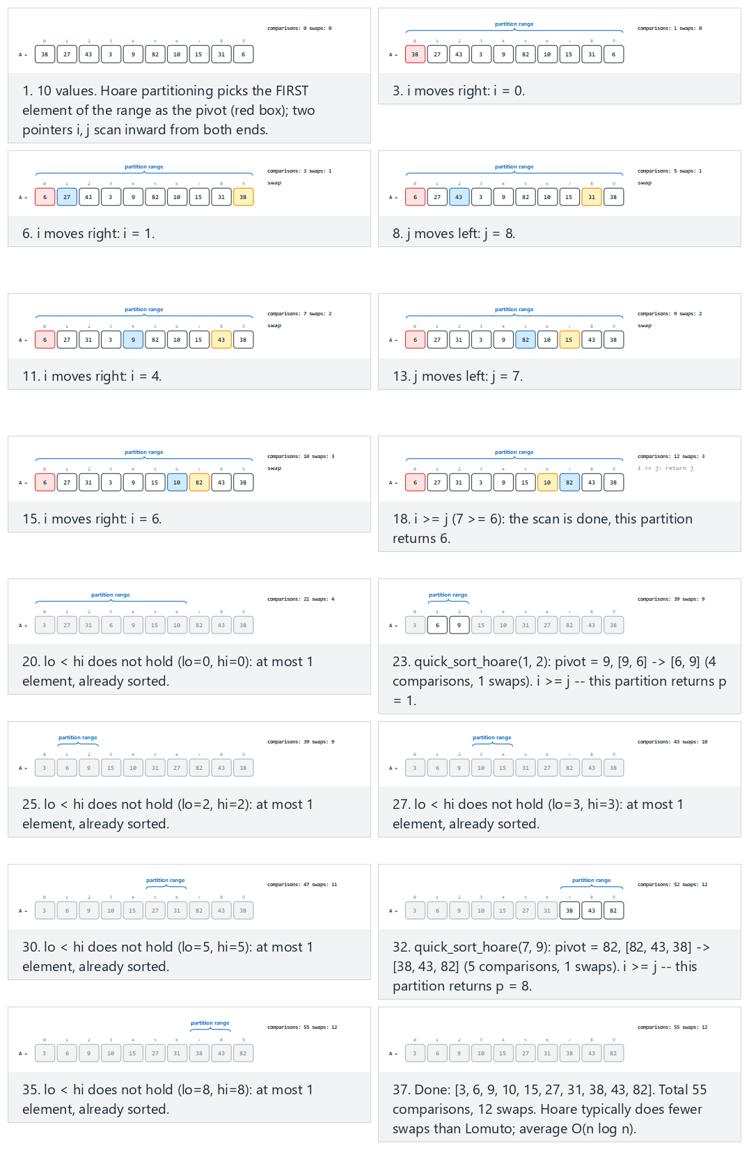
In the picker, also try repeated keys and compare its total swap count against Lomuto's on the identical input (section 7.6 discusses why Hoare typically does fewer swaps), or press 🎲 for random data, or type your own array.
Full program: quick_sort_hoare.c / QuickSortHoare.java
/* Week 10 -- Sorting
 * Quick sort with Hoare partitioning: pivot = first element of the range.
 * Two pointers scan inward from both ends and swap out-of-place pairs; the
 * partition does NOT guarantee the pivot itself lands at the returned
 * index. Recursive calls are (lo, p) and (p + 1, hi) -- note p, not
 * p - 1. Prints every partition call and the total comparisons/swaps.
 * CEN207 Data Structures (formerly CE205)
 */
#include <stdio.h>

static int comparisons, swaps;

static void print_range(const int a[], int lo, int hi) {
    printf("[");
    for (int i = lo; i <= hi; i++) printf("%d%s", a[i], i < hi ? "," : "");
    printf("]");
}

int partition_hoare(int a[], int lo, int hi) {
    int pivot = a[lo];
    int i = lo - 1, j = hi + 1;
    while (1) {
        do { i++; comparisons++; } while (a[i] < pivot);
        do { j--; comparisons++; } while (a[j] > pivot);
        if (i >= j) return j;
        int tmp = a[i]; a[i] = a[j]; a[j] = tmp;
        swaps++;
    }
}

void quick_sort_hoare(int a[], int lo, int hi) {
    if (lo < hi) {
        printf("  partition [%d..%d] ", lo, hi);
        print_range(a, lo, hi);
        printf(" pivot=%d -> ", a[lo]);
        int p = partition_hoare(a, lo, hi);
        print_range(a, lo, hi);
        printf(" (returns %d)\n", p);
        quick_sort_hoare(a, lo, p);
        quick_sort_hoare(a, p + 1, hi);
    }
}

static void print_array(const int a[], int n) { print_range(a, 0, n - 1); printf("\n"); }

static void run_scenario(const char *label, int a[], int n) {
    printf("-- %s --\n", label);
    printf("before: ");
    print_array(a, n);
    comparisons = 0; swaps = 0;
    quick_sort_hoare(a, 0, n - 1);
    printf("after:  ");
    print_array(a, n);
    printf("total: %d comparisons, %d swaps\n\n", comparisons, swaps);
}

int main(void) {
    int normal[] = {38, 27, 43, 3, 9, 82, 10, 15, 31, 6};
    int repeated[] = {7, 2, 7, 9, 2, 7, 4, 9, 2, 4, 7, 9};
    int already_sorted[] = {1, 2, 3, 4, 5, 6, 7, 8, 9, 10};
    int reverse_sorted[] = {10, 9, 8, 7, 6, 5, 4, 3, 2, 1};

    run_scenario("normal: 10 unordered values", normal, 10);
    run_scenario("hard: 12 values with repeated keys", repeated, 12);
    run_scenario("edge: already sorted -- every scan still runs", already_sorted, 10);
    run_scenario("edge: reverse sorted -- worst case", reverse_sorted, 10);

    return 0;
}
/* Week 10 -- Sorting
 * Quick sort with Hoare partitioning: pivot = first element of the range.
 * Two pointers scan inward from both ends and swap out-of-place pairs; the
 * partition does NOT guarantee the pivot itself lands at the returned
 * index. Recursive calls are (lo, p) and (p + 1, hi) -- note p, not
 * p - 1. Prints every partition call and the total comparisons/swaps.
 * CEN207 Data Structures (formerly CE205)
 */
public class QuickSortHoare {
    static int comparisons, swaps;

    static String rangeStr(int[] a, int lo, int hi) {
        StringBuilder sb = new StringBuilder("[");
        for (int i = lo; i <= hi; i++) { sb.append(a[i]); if (i < hi) sb.append(','); }
        sb.append(']');
        return sb.toString();
    }

    static int partitionHoare(int[] a, int lo, int hi) {
        int pivot = a[lo];
        int i = lo - 1, j = hi + 1;
        while (true) {
            do { i++; comparisons++; } while (a[i] < pivot);
            do { j--; comparisons++; } while (a[j] > pivot);
            if (i >= j) return j;
            int tmp = a[i]; a[i] = a[j]; a[j] = tmp;
            swaps++;
        }
    }

    static void quickSortHoare(int[] a, int lo, int hi) {
        if (lo < hi) {
            String before = rangeStr(a, lo, hi);
            int pivotVal = a[lo];
            int p = partitionHoare(a, lo, hi);
            System.out.println("  partition [" + lo + ".." + hi + "] " + before + " pivot=" + pivotVal + " -> " + rangeStr(a, lo, hi) + " (returns " + p + ")");
            quickSortHoare(a, lo, p);
            quickSortHoare(a, p + 1, hi);
        }
    }

    static void printArray(int[] a) { System.out.println(rangeStr(a, 0, a.length - 1)); }

    static void runScenario(String label, int[] a) {
        System.out.println("-- " + label + " --");
        System.out.print("before: ");
        printArray(a);
        comparisons = 0; swaps = 0;
        quickSortHoare(a, 0, a.length - 1);
        System.out.print("after:  ");
        printArray(a);
        System.out.println("total: " + comparisons + " comparisons, " + swaps + " swaps");
        System.out.println();
    }

    public static void main(String[] args) {
        int[] normal = {38, 27, 43, 3, 9, 82, 10, 15, 31, 6};
        int[] repeated = {7, 2, 7, 9, 2, 7, 4, 9, 2, 4, 7, 9};
        int[] alreadySorted = {1, 2, 3, 4, 5, 6, 7, 8, 9, 10};
        int[] reverseSorted = {10, 9, 8, 7, 6, 5, 4, 3, 2, 1};

        runScenario("normal: 10 unordered values", normal);
        runScenario("hard: 12 values with repeated keys", repeated);
        runScenario("edge: already sorted -- every scan still runs", alreadySorted);
        runScenario("edge: reverse sorted -- worst case", reverseSorted);
    }
}
Try it
Expected output:
-- normal: 10 unordered values --
before: [38,27,43,3,9,82,10,15,31,6]
  partition [0..9] [38,27,43,3,9,82,10,15,31,6] pivot=38 -> [6,27,31,3,9,15,10,82,43,38] (returns 6)
  partition [0..6] [6,27,31,3,9,15,10] pivot=6 -> [3,27,31,6,9,15,10] (returns 0)
  partition [1..6] [27,31,6,9,15,10] pivot=27 -> [10,15,6,9,31,27] (returns 4)
  partition [1..4] [10,15,6,9] pivot=10 -> [9,6,15,10] (returns 2)
  partition [1..2] [9,6] pivot=9 -> [6,9] (returns 1)
  partition [3..4] [15,10] pivot=15 -> [10,15] (returns 3)
  partition [5..6] [31,27] pivot=31 -> [27,31] (returns 5)
  partition [7..9] [82,43,38] pivot=82 -> [38,43,82] (returns 8)
  partition [7..8] [38,43] pivot=38 -> [38,43] (returns 7)
after:  [3,6,9,10,15,27,31,38,43,82]
total: 55 comparisons, 12 swaps

-- hard: 12 values with repeated keys --
before: [7,2,7,9,2,7,4,9,2,4,7,9]
  partition [0..11] [7,2,7,9,2,7,4,9,2,4,7,9] pivot=7 -> [7,2,4,2,2,4,7,9,9,7,7,9] (returns 5)
  partition [0..5] [7,2,4,2,2,4] pivot=7 -> [4,2,4,2,2,7] (returns 4)
  partition [0..4] [4,2,4,2,2] pivot=4 -> [2,2,2,4,4] (returns 2)
  partition [0..2] [2,2,2] pivot=2 -> [2,2,2] (returns 1)
  partition [0..1] [2,2] pivot=2 -> [2,2] (returns 0)
  partition [3..4] [4,4] pivot=4 -> [4,4] (returns 3)
  partition [6..11] [7,9,9,7,7,9] pivot=7 -> [7,7,9,9,7,9] (returns 7)
  partition [6..7] [7,7] pivot=7 -> [7,7] (returns 6)
  partition [8..11] [9,9,7,9] pivot=9 -> [9,7,9,9] (returns 9)
  partition [8..9] [9,7] pivot=9 -> [7,9] (returns 8)
  partition [10..11] [9,9] pivot=9 -> [9,9] (returns 10)
after:  [2,2,2,4,4,7,7,7,7,9,9,9]
total: 67 comparisons, 17 swaps

-- edge: already sorted -- every scan still runs --
before: [1,2,3,4,5,6,7,8,9,10]
  partition [0..9] [1,2,3,4,5,6,7,8,9,10] pivot=1 -> [1,2,3,4,5,6,7,8,9,10] (returns 0)
  partition [1..9] [2,3,4,5,6,7,8,9,10] pivot=2 -> [2,3,4,5,6,7,8,9,10] (returns 1)
  partition [2..9] [3,4,5,6,7,8,9,10] pivot=3 -> [3,4,5,6,7,8,9,10] (returns 2)
  partition [3..9] [4,5,6,7,8,9,10] pivot=4 -> [4,5,6,7,8,9,10] (returns 3)
  partition [4..9] [5,6,7,8,9,10] pivot=5 -> [5,6,7,8,9,10] (returns 4)
  partition [5..9] [6,7,8,9,10] pivot=6 -> [6,7,8,9,10] (returns 5)
  partition [6..9] [7,8,9,10] pivot=7 -> [7,8,9,10] (returns 6)
  partition [7..9] [8,9,10] pivot=8 -> [8,9,10] (returns 7)
  partition [8..9] [9,10] pivot=9 -> [9,10] (returns 8)
after:  [1,2,3,4,5,6,7,8,9,10]
total: 63 comparisons, 0 swaps

-- edge: reverse sorted -- worst case --
before: [10,9,8,7,6,5,4,3,2,1]
  partition [0..9] [10,9,8,7,6,5,4,3,2,1] pivot=10 -> [1,9,8,7,6,5,4,3,2,10] (returns 8)
  partition [0..8] [1,9,8,7,6,5,4,3,2] pivot=1 -> [1,9,8,7,6,5,4,3,2] (returns 0)
  partition [1..8] [9,8,7,6,5,4,3,2] pivot=9 -> [2,8,7,6,5,4,3,9] (returns 7)
  partition [1..7] [2,8,7,6,5,4,3] pivot=2 -> [2,8,7,6,5,4,3] (returns 1)
  partition [2..7] [8,7,6,5,4,3] pivot=8 -> [3,7,6,5,4,8] (returns 6)
  partition [2..6] [3,7,6,5,4] pivot=3 -> [3,7,6,5,4] (returns 2)
  partition [3..6] [7,6,5,4] pivot=7 -> [4,6,5,7] (returns 5)
  partition [3..5] [4,6,5] pivot=4 -> [4,6,5] (returns 3)
  partition [4..5] [6,5] pivot=6 -> [5,6] (returns 4)
after:  [1,2,3,4,5,6,7,8,9,10]
total: 68 comparisons, 5 swaps
7.5 The worst case, and how pivot choice avoids it
Both schemes above always pick a fixed corner element (Lomuto: last; Hoare: first) as the pivot. Look back at Lomuto's "already sorted" run: every single partition split n-1 elements against 0 — the worst possible split, giving O(n^2) instead of O(n log n). This is not a coincidence of that one example; it is what always happens when the pivot always turns out to be the smallest or largest remaining element, which is exactly what "always pick the first/last element" guarantees on already-sorted or reverse-sorted input.
quick-sort-worst-case runs the identical input through the identical Lomuto-style partition three times, changing only how the pivot is chosen: always the first element (the classic trap); the middle index; and the median of the first, middle, and last elements ("median-of-three"), the standard real-world defense. All three still use exactly the same partitioning mechanic from section 7.3 — only the one line that picks pivot_idx changes.
void swap(int a[], int x, int y) { int t = a[x]; a[x] = a[y]; a[y] = t; }

int choose_pivot_first(int a[], int lo, int hi)  { return lo; }
int choose_pivot_middle(int a[], int lo, int hi) { return (lo + hi) / 2; }
int choose_pivot_median3(int a[], int lo, int hi) {
    int mid = (lo + hi) / 2;
    if (a[mid] < a[lo]) swap(a, lo, mid);
    if (a[hi] < a[lo])  swap(a, lo, hi);
    if (a[hi] < a[mid]) swap(a, mid, hi);
    return mid;                    /* the median of the three now sits at mid */
}

int partition_with(int a[], int lo, int hi, int pivot_idx) {
    swap(a, pivot_idx, hi);        /* move the chosen pivot to the end, then run Lomuto */
    int pivot = a[hi];
    int i = lo - 1;
    for (int j = lo; j < hi; j++)
        if (a[j] <= pivot) { i++; swap(a, i, j); }
    swap(a, i + 1, hi);
    return i + 1;
}
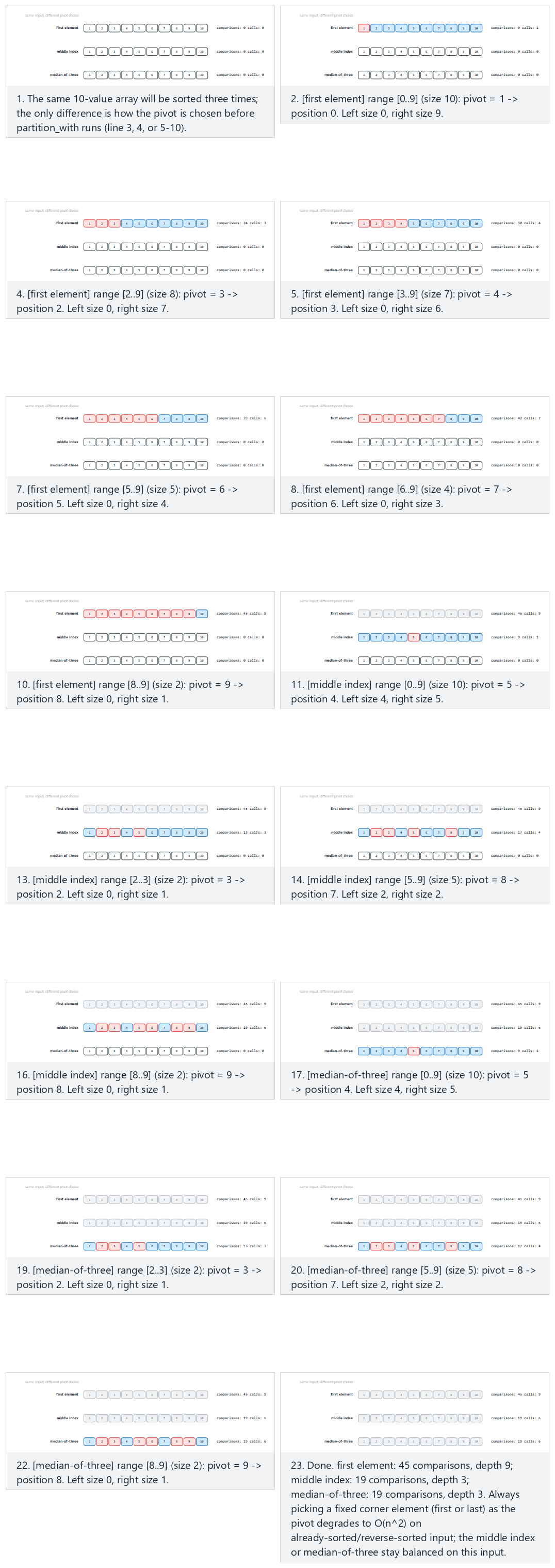
In the picker, the default example is exactly this trap: already sorted, first-element is the worst case. Also try random — all three strategies are similar (when the input has no adversarial structure, even the naive fixed-corner pivot does fine on average), or type your own array.
Full program: quick_sort_worst_case.c / QuickSortWorstCase.java
/* Week 10 -- Sorting
 * Quick sort's worst case, and how pivot choice avoids it: the SAME input
 * is sorted three times with the same Lomuto-style partition, differing
 * only in which element is chosen as the pivot (first / middle / median-
 * of-three). Prints each strategy's total comparisons and recursion depth
 * on the same input, so the O(n^2) vs O(n log n) gap becomes a number.
 * CEN207 Data Structures (formerly CE205)
 */
#include <stdio.h>

static void swap(int a[], int x, int y) { int t = a[x]; a[x] = a[y]; a[y] = t; }

static int choose_pivot_first(int a[], int lo, int hi) { (void) a; (void) hi; return lo; }
static int choose_pivot_middle(int a[], int lo, int hi) { (void) a; return lo + (hi - lo) / 2; }
static int choose_pivot_median3(int a[], int lo, int hi) {
    int mid = lo + (hi - lo) / 2;
    if (a[mid] < a[lo]) swap(a, lo, mid);
    if (a[hi] < a[lo]) swap(a, lo, hi);
    if (a[hi] < a[mid]) swap(a, mid, hi);
    return mid;
}

static int partition_with(int a[], int lo, int hi, int pivot_idx, int *comparisons) {
    swap(a, pivot_idx, hi);
    int pivot = a[hi];
    int i = lo - 1;
    for (int j = lo; j < hi; j++) {
        (*comparisons)++;
        if (a[j] <= pivot) { i++; swap(a, i, j); }
    }
    swap(a, i + 1, hi);
    return i + 1;
}

typedef int (*PivotFn)(int[], int, int);

static void qs(int a[], int lo, int hi, PivotFn pick, int *comparisons, int *calls, int depth, int *max_depth) {
    if (depth > *max_depth) *max_depth = depth;
    if (hi <= lo) return;
    (*calls)++;
    int p_idx = pick(a, lo, hi);
    int p = partition_with(a, lo, hi, p_idx, comparisons);
    qs(a, lo, p - 1, pick, comparisons, calls, depth + 1, max_depth);
    qs(a, p + 1, hi, pick, comparisons, calls, depth + 1, max_depth);
}

static void print_array(const int a[], int n) {
    printf("[");
    for (int i = 0; i < n; i++) printf("%d%s", a[i], i + 1 < n ? "," : "");
    printf("]\n");
}

static void run_strategy(const char *name, const int src[], int n, PivotFn pick) {
    int a[32];
    for (int i = 0; i < n; i++) a[i] = src[i];
    int comparisons = 0, calls = 0, max_depth = 0;
    qs(a, 0, n - 1, pick, &comparisons, &calls, 0, &max_depth);
    printf("  %-16s comparisons=%-4d calls=%-3d depth=%-3d -> ", name, comparisons, calls, max_depth);
    print_array(a, n);
}

static void run_scenario(const char *label, const int a[], int n) {
    printf("-- %s --\n", label);
    printf("before: ");
    print_array(a, n);
    run_strategy("first element", a, n, choose_pivot_first);
    run_strategy("middle index", a, n, choose_pivot_middle);
    run_strategy("median-of-3", a, n, choose_pivot_median3);
    printf("\n");
}

int main(void) {
    int sorted10[] = {1, 2, 3, 4, 5, 6, 7, 8, 9, 10};
    int sorted14[] = {1, 2, 3, 4, 5, 6, 7, 8, 9, 10, 11, 12, 13, 14};
    int reverse10[] = {10, 9, 8, 7, 6, 5, 4, 3, 2, 1};
    int random10[] = {38, 27, 43, 3, 9, 82, 10, 15, 31, 6};

    run_scenario("normal: already-sorted 10 values -- first-element is the worst case", sorted10, 10);
    run_scenario("hard: already-sorted 14 values -- the gap widens further", sorted14, 14);
    run_scenario("edge: reverse-sorted 10 values -- first-element is again the worst case", reverse10, 10);
    run_scenario("edge: random 10 values -- all three strategies are similar", random10, 10);

    return 0;
}
/* Week 10 -- Sorting
 * Quick sort's worst case, and how pivot choice avoids it: the SAME input
 * is sorted three times with the same Lomuto-style partition, differing
 * only in which element is chosen as the pivot (first / middle / median-
 * of-three). Prints each strategy's total comparisons and recursion depth
 * on the same input, so the O(n^2) vs O(n log n) gap becomes a number.
 * CEN207 Data Structures (formerly CE205)
 */
public class QuickSortWorstCase {
    interface Pivot { int pick(int[] a, int lo, int hi); }

    static void swap(int[] a, int x, int y) { int t = a[x]; a[x] = a[y]; a[y] = t; }

    static int choosePivotFirst(int[] a, int lo, int hi) { return lo; }
    static int choosePivotMiddle(int[] a, int lo, int hi) { return lo + (hi - lo) / 2; }
    static int choosePivotMedian3(int[] a, int lo, int hi) {
        int mid = lo + (hi - lo) / 2;
        if (a[mid] < a[lo]) swap(a, lo, mid);
        if (a[hi] < a[lo]) swap(a, lo, hi);
        if (a[hi] < a[mid]) swap(a, mid, hi);
        return mid;
    }

    static int[] comparisons = new int[1];
    static int[] calls = new int[1];
    static int[] maxDepth = new int[1];

    static int partitionWith(int[] a, int lo, int hi, int pivotIdx) {
        swap(a, pivotIdx, hi);
        int pivot = a[hi];
        int i = lo - 1;
        for (int j = lo; j < hi; j++) {
            comparisons[0]++;
            if (a[j] <= pivot) { i++; swap(a, i, j); }
        }
        swap(a, i + 1, hi);
        return i + 1;
    }

    static void qs(int[] a, int lo, int hi, Pivot pick, int depth) {
        if (depth > maxDepth[0]) maxDepth[0] = depth;
        if (hi <= lo) return;
        calls[0]++;
        int pIdx = pick.pick(a, lo, hi);
        int p = partitionWith(a, lo, hi, pIdx);
        qs(a, lo, p - 1, pick, depth + 1);
        qs(a, p + 1, hi, pick, depth + 1);
    }

    static void printArray(int[] a) {
        StringBuilder sb = new StringBuilder("[");
        for (int i = 0; i < a.length; i++) { sb.append(a[i]); if (i + 1 < a.length) sb.append(','); }
        sb.append(']');
        System.out.println(sb);
    }

    static void runStrategy(String name, int[] src, Pivot pick) {
        int[] a = src.clone();
        comparisons[0] = 0; calls[0] = 0; maxDepth[0] = 0;
        qs(a, 0, a.length - 1, pick, 0);
        System.out.printf("  %-16s comparisons=%-4d calls=%-3d depth=%-3d -> ", name, comparisons[0], calls[0], maxDepth[0]);
        printArray(a);
    }

    static void runScenario(String label, int[] a) {
        System.out.println("-- " + label + " --");
        System.out.print("before: ");
        printArray(a);
        runStrategy("first element", a, QuickSortWorstCase::choosePivotFirst);
        runStrategy("middle index", a, QuickSortWorstCase::choosePivotMiddle);
        runStrategy("median-of-3", a, QuickSortWorstCase::choosePivotMedian3);
        System.out.println();
    }

    public static void main(String[] args) {
        int[] sorted10 = {1, 2, 3, 4, 5, 6, 7, 8, 9, 10};
        int[] sorted14 = {1, 2, 3, 4, 5, 6, 7, 8, 9, 10, 11, 12, 13, 14};
        int[] reverse10 = {10, 9, 8, 7, 6, 5, 4, 3, 2, 1};
        int[] random10 = {38, 27, 43, 3, 9, 82, 10, 15, 31, 6};

        runScenario("normal: already-sorted 10 values -- first-element is the worst case", sorted10);
        runScenario("hard: already-sorted 14 values -- the gap widens further", sorted14);
        runScenario("edge: reverse-sorted 10 values -- first-element is again the worst case", reverse10);
        runScenario("edge: random 10 values -- all three strategies are similar", random10);
    }
}
Try it
Expected output:
-- normal: already-sorted 10 values -- first-element is the worst case --
before: [1,2,3,4,5,6,7,8,9,10]
  first element    comparisons=45   calls=9   depth=9   -> [1,2,3,4,5,6,7,8,9,10]
  middle index     comparisons=19   calls=6   depth=3   -> [1,2,3,4,5,6,7,8,9,10]
  median-of-3      comparisons=19   calls=6   depth=3   -> [1,2,3,4,5,6,7,8,9,10]

-- hard: already-sorted 14 values -- the gap widens further --
before: [1,2,3,4,5,6,7,8,9,10,11,12,13,14]
  first element    comparisons=91   calls=13  depth=13  -> [1,2,3,4,5,6,7,8,9,10,11,12,13,14]
  middle index     comparisons=31   calls=7   depth=3   -> [1,2,3,4,5,6,7,8,9,10,11,12,13,14]
  median-of-3      comparisons=31   calls=7   depth=3   -> [1,2,3,4,5,6,7,8,9,10,11,12,13,14]

-- edge: reverse-sorted 10 values -- first-element is again the worst case --
before: [10,9,8,7,6,5,4,3,2,1]
  first element    comparisons=45   calls=9   depth=9   -> [1,2,3,4,5,6,7,8,9,10]
  middle index     comparisons=21   calls=6   depth=4   -> [1,2,3,4,5,6,7,8,9,10]
  median-of-3      comparisons=19   calls=5   depth=3   -> [1,2,3,4,5,6,7,8,9,10]

-- edge: random 10 values -- all three strategies are similar --
before: [38,27,43,3,9,82,10,15,31,6]
  first element    comparisons=26   calls=7   depth=6   -> [3,6,9,10,15,27,31,38,43,82]
  middle index     comparisons=27   calls=7   depth=6   -> [3,6,9,10,15,27,31,38,43,82]
  median-of-3      comparisons=21   calls=6   depth=4   -> [3,6,9,10,15,27,31,38,43,82]
Look at the "already sorted, 14 values" numbers: the first-element strategy needed 91 comparisons and a recursion depth of 13 (one level deeper for every single element — exactly the degenerate, linked-list-like recursion a bad pivot produces); the middle-index and median-of-three strategies needed only 31 comparisons and a depth of 3 on the identical input. That gap — 91 versus 31 — is O(n^2) versus O(n log n) made concrete.
7.6 Complexity, mistakes, self-check
Complexity. Average case O(n log n), and in practice the fastest of the comparison-based sorts this week for large random data, due to good cache behavior and a small constant factor — real-world library sorts (C's qsort, and historically Java's primitive-array sort) are quick sort variants for exactly this reason. Worst case O(n^2), whenever the pivot choice consistently produces a badly unbalanced split — section 7.5 showed this happening for both Lomuto and Hoare's fixed-corner pivots on sorted/reverse-sorted input. A single theoretical fact ties every comparison-based sort in this course together: no comparison-based sorting algorithm can guarantee better than O(n log n) comparisons in the worst case — there are n! possible orderings of n distinct elements, a decision tree of yes/no comparisons that distinguishes all of them needs at least log2(n!) levels, and log2(n!) is O(n log n) by Stirling's approximation (you will prove this bound for yourself as an exercise). Merge sort meets that bound exactly, in every case; quick sort meets it only on average. Space: Lomuto and Hoare partitioning are both O(1) extra per partition call, but the recursion itself uses O(log n) stack space on average (O(n) in the worst case, matching the comparison blow-up). Quick sort is NOT stable: both partitioning schemes swap elements across long distances with no regard for ties (see section 11).
Common mistakes
- Mixing up Lomuto's
p - 1/p + 1recursion with Hoare'sp/p + 1. This is the single most common quick-sort bug. Lomuto's partition guarantees the pivot sits exactly at the returned indexp, so both sub-ranges must exclude it (lo, p-1andp+1, hi). Hoare's partition makes no such guarantee about the pivot's final position, so recursing onlo, p-1can drop an element that still needs sorting — the correct calls arelo, pandp+1, hi, as shown in section 7.4's code. - Forgetting the base case
lo < hi(Lomuto) / equivalent guard, or writinglo <= hi, which recurses forever on a single-element range (lo == hishould simply return, since one element is already sorted). - Choosing a pivot that ignores the input's structure, i.e., always the first or last element with no randomization or median-of-three defense, on data that might realistically already be sorted or nearly so (log files, timestamped records, re-sorting after a small update) — exactly the adversarial case section 7.5 demonstrates numerically.
Self-check: the comparison-sorting lower bound
There are n! distinct orderings of n distinct elements. A comparison-based sort must, in the worst case, distinguish every one of these orderings using only pairwise (<, >, =) comparisons. Explain why this forces at least log2(n!) comparisons in the worst case, and why log2(n!) is O(n log n).
Answer. Model every possible execution of a comparison-based sort as a binary decision tree: each internal node is one comparison, each leaf is one final, fully determined ordering of the output. Since the algorithm must be able to correctly sort any of the n! possible input orderings, the tree must have at least n! distinct leaves — and a binary tree with L leaves needs a height of at least log2(L), so the worst-case number of comparisons (the height of the tree) is at least log2(n!). By Stirling's approximation, log2(n!) = n*log2(n) - n*log2(e) + O(log n), whose dominant term is n*log2(n) — so log2(n!) is O(n log n), and no comparison-based sort can ever guarantee fewer comparisons than that in the worst case, no matter how cleverly it is designed.
8. Counting sort
8.1 A question to start
Section 7.6 proved that comparison-based sorting can never guarantee better than O(n log n). That proof has a hidden assumption, though: it assumes the only thing you know about a value is how it compares to another value. What if you know more — say, that every value is a small non-negative integer? Then you do not need to compare keys at all: you can simply count how many times each possible value occurs. Harold H. Seward described this idea in his 1954 master's thesis at MIT, and it remains the simplest way to beat the comparison lower bound, whenever it applies.
8.2 The idea: count, accumulate, place
For values known to lie in 0..maxVal: first, build count[] of size maxVal + 1 and count how many times each value occurs (count[v]++ for every a[i] == v). Second, turn those raw counts into a cumulative sum, count[v] += count[v-1], so that count[v] now means "how many values are <= v" — which is exactly the last (rightmost) index that value v should occupy in the sorted output. Third, place every input value directly into output[count[a[i]] - 1], decrementing count[a[i]] afterward so the next occurrence of that same value lands one slot earlier. Scanning the input backwards in this last step is what keeps the sort stable: it guarantees that among several equal values, the one that appeared earlier in the input lands in the earlier of their reserved output slots.
8.3 In memory, and the code
void counting_sort(int a[], int n, int max_val) {
    int count[max_val + 1];
    for (int v = 0; v <= max_val; v++) count[v] = 0;
    for (int i = 0; i < n; i++) count[a[i]]++;          /* raw counts */
    for (int v = 1; v <= max_val; v++) count[v] += count[v - 1];   /* cumulative */
    int output[n];
    for (int i = n - 1; i >= 0; i--) {                  /* backwards: keeps it stable */
        output[count[a[i]] - 1] = a[i];
        count[a[i]]--;
    }
    for (int i = 0; i < n; i++) a[i] = output[i];
}
void countingSort(int[] a, int n, int maxVal) {
    int[] count = new int[maxVal + 1];
    for (int v = 0; v <= maxVal; v++) count[v] = 0;
    for (int i = 0; i < n; i++) count[a[i]]++;          // raw counts
    for (int v = 1; v <= maxVal; v++) count[v] += count[v - 1];   // cumulative
    int[] output = new int[n];
    for (int i = n - 1; i >= 0; i--) {                  // backwards: keeps it stable
        output[count[a[i]] - 1] = a[i];
        count[a[i]]--;
    }
    for (int i = 0; i < n; i++) a[i] = output[i];
}
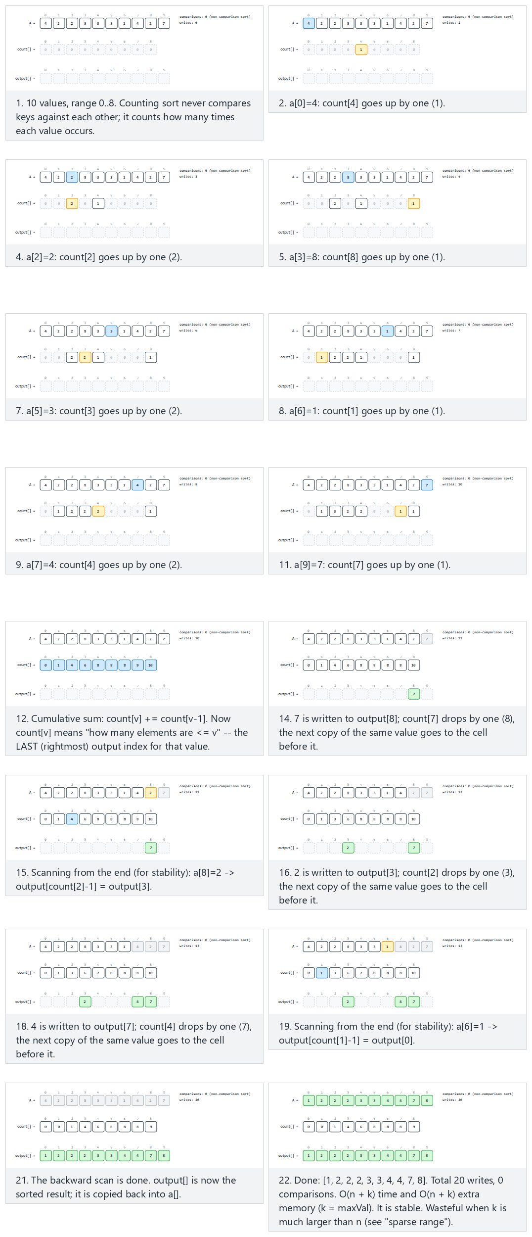
Watch the counters on the right: comparisons stays at 0 throughout — that is the entire point of a non-comparison sort, not an animation bug. In the picker, also try sparse range — 10 values but maxVal=15 (the O(n + k) cost made concrete: the count[] row has to cover every value up to 15 even though only 10 of those slots are ever used), or press 🎲 for random data, or type your own array of values in 0..15.
8.4 Try it
Full program: counting_sort.c / CountingSort.java
/* Week 10 -- Sorting
 * Counting sort: a non-comparison sort for small non-negative integers.
 * Counts occurrences of each value, turns the counts into a cumulative
 * total, then places every input value directly at its final index,
 * scanning backwards to stay stable. Prints count[] at each stage and the
 * final result. Zero comparisons; the total writes are reported.
 * CEN207 Data Structures (formerly CE205)
 */
#include <stdio.h>

static void print_array(const int a[], int n) {
    printf("[");
    for (int i = 0; i < n; i++) printf("%d%s", a[i], i + 1 < n ? "," : "");
    printf("]\n");
}

void counting_sort(int a[], int n, int max_val, int *writes) {
    int count[64] = {0};
    for (int i = 0; i < n; i++) { count[a[i]]++; (*writes)++; }
    printf("  raw counts:        ");
    print_array(count, max_val + 1);
    for (int v = 1; v <= max_val; v++) count[v] += count[v - 1];
    printf("  cumulative counts: ");
    print_array(count, max_val + 1);

    int output[64];
    for (int i = n - 1; i >= 0; i--) {
        output[count[a[i]] - 1] = a[i];
        (*writes)++;
        count[a[i]]--;
    }
    for (int i = 0; i < n; i++) a[i] = output[i];
}

static void run_scenario(const char *label, int a[], int n, int max_val) {
    printf("-- %s --\n", label);
    printf("before: ");
    print_array(a, n);
    int writes = 0;
    counting_sort(a, n, max_val, &writes);
    printf("after:  ");
    print_array(a, n);
    printf("total: 0 comparisons, %d writes\n\n", writes);
}

int main(void) {
    int normal[] = {4, 2, 2, 8, 3, 3, 1, 4, 2, 7};
    int hard[] = {5, 1, 5, 9, 2, 5, 1, 9, 5, 2, 1, 9, 5, 0};
    int already_sorted[] = {0, 1, 2, 3, 4, 5, 6, 7, 8, 9};
    int sparse[] = {0, 15, 3, 12, 6, 9, 1, 14, 7, 8};

    run_scenario("normal: 10 values, range 0..9", normal, 10, 9);
    run_scenario("hard: 14 values, range 0..9, heavy repeats", hard, 14, 9);
    run_scenario("edge: already sorted -- every pass still runs", already_sorted, 10, 9);
    run_scenario("edge: sparse range -- 10 values but maxVal=15 (the O(n+k) cost)", sparse, 10, 15);

    return 0;
}
/* Week 10 -- Sorting
 * Counting sort: a non-comparison sort for small non-negative integers.
 * Counts occurrences of each value, turns the counts into a cumulative
 * total, then places every input value directly at its final index,
 * scanning backwards to stay stable. Prints count[] at each stage and the
 * final result. Zero comparisons; the total writes are reported.
 * CEN207 Data Structures (formerly CE205)
 */
public class CountingSort {
    static void printArray(int[] a, int n) {
        StringBuilder sb = new StringBuilder("[");
        for (int i = 0; i < n; i++) { sb.append(a[i]); if (i + 1 < n) sb.append(','); }
        sb.append(']');
        System.out.println(sb);
    }

    static int countingSort(int[] a, int n, int maxVal) {
        int writes = 0;
        int[] count = new int[maxVal + 1];
        for (int i = 0; i < n; i++) { count[a[i]]++; writes++; }
        System.out.print("  raw counts:        ");
        printArray(count, maxVal + 1);
        for (int v = 1; v <= maxVal; v++) count[v] += count[v - 1];
        System.out.print("  cumulative counts: ");
        printArray(count, maxVal + 1);

        int[] output = new int[n];
        for (int i = n - 1; i >= 0; i--) {
            output[count[a[i]] - 1] = a[i];
            writes++;
            count[a[i]]--;
        }
        for (int i = 0; i < n; i++) a[i] = output[i];
        return writes;
    }

    static void runScenario(String label, int[] a, int maxVal) {
        System.out.println("-- " + label + " --");
        System.out.print("before: ");
        printArray(a, a.length);
        int writes = countingSort(a, a.length, maxVal);
        System.out.print("after:  ");
        printArray(a, a.length);
        System.out.println("total: 0 comparisons, " + writes + " writes");
        System.out.println();
    }

    public static void main(String[] args) {
        int[] normal = {4, 2, 2, 8, 3, 3, 1, 4, 2, 7};
        int[] hard = {5, 1, 5, 9, 2, 5, 1, 9, 5, 2, 1, 9, 5, 0};
        int[] alreadySorted = {0, 1, 2, 3, 4, 5, 6, 7, 8, 9};
        int[] sparse = {0, 15, 3, 12, 6, 9, 1, 14, 7, 8};

        runScenario("normal: 10 values, range 0..9", normal, 9);
        runScenario("hard: 14 values, range 0..9, heavy repeats", hard, 9);
        runScenario("edge: already sorted -- every pass still runs", alreadySorted, 9);
        runScenario("edge: sparse range -- 10 values but maxVal=15 (the O(n+k) cost)", sparse, 15);
    }
}
Try it
Expected output:
-- normal: 10 values, range 0..9 --
before: [4,2,2,8,3,3,1,4,2,7]
  raw counts:        [0,1,3,2,2,0,0,1,1,0]
  cumulative counts: [0,1,4,6,8,8,8,9,10,10]
after:  [1,2,2,2,3,3,4,4,7,8]
total: 0 comparisons, 20 writes

-- hard: 14 values, range 0..9, heavy repeats --
before: [5,1,5,9,2,5,1,9,5,2,1,9,5,0]
  raw counts:        [1,3,2,0,0,5,0,0,0,3]
  cumulative counts: [1,4,6,6,6,11,11,11,11,14]
after:  [0,1,1,1,2,2,5,5,5,5,5,9,9,9]
total: 0 comparisons, 28 writes

-- edge: already sorted -- every pass still runs --
before: [0,1,2,3,4,5,6,7,8,9]
  raw counts:        [1,1,1,1,1,1,1,1,1,1]
  cumulative counts: [1,2,3,4,5,6,7,8,9,10]
after:  [0,1,2,3,4,5,6,7,8,9]
total: 0 comparisons, 20 writes

-- edge: sparse range -- 10 values but maxVal=15 (the O(n+k) cost) --
before: [0,15,3,12,6,9,1,14,7,8]
  raw counts:        [1,1,0,1,0,0,1,1,1,1,0,0,1,0,1,1]
  cumulative counts: [1,2,2,3,3,3,4,5,6,7,7,7,8,8,9,10]
after:  [0,1,3,6,7,8,9,12,14,15]
total: 0 comparisons, 20 writes
8.5 Complexity, mistakes, self-check
Complexity. O(n + k) time, where k = maxVal, in every case — the array is scanned a small, fixed number of times, with no dependence on the input's order at all. O(n + k) extra space, for count[] and output[]. This is genuinely better than any comparison-based sort's O(n log n) bound when k is not much larger than n — but look at the sparse-range example above: k = 15 for only n = 10 values, so the extra memory (and the work of zeroing/scanning count[]) is already comparable to n itself; for k much larger than n (say, sorting 10 values drawn from 0..1000000), counting sort becomes wildly wasteful, allocating and scanning a million-entry array to sort ten numbers. Counting sort is stable — by design, via the backwards final scan (section 8.2).
Common mistakes
- Scanning forward instead of backward in the placement step. Counting sort is still numerically correct either way (the multiset of output values is the same), but stability is lost — always scan backwards for a stable ascending counting sort.
- Using counting sort on data with a large or unbounded range, or on floating-point or non-integer keys, where it does not apply at all — counting sort's
O(n + k)guarantee is only good whenkstays small relative ton; radix sort (section 9) rescues the idea for larger integers by applying counting sort one digit at a time instead of over the whole value range at once. - Off-by-one on
count[]'s size or the cumulative-sum loop bounds.count[]needsmaxVal + 1entries (indices0..maxVal), and the cumulative sum starts atv = 1(count[0]is already correct as its own raw count) — an easy place to introduce a silent out-of-bounds write.
Self-check: why does the backward scan preserve stability?
Two equal values a[p] and a[q], with p < q (so a[p] appears earlier in the input), both have the same key v and are therefore both entitled to consecutive slots in output[]. Trace through the backward-scanning placement step and explain why a[p] always ends up to the LEFT of a[q] in the output, never the right.
Answer. The scan processes a[q] before a[p] (since q > p and the loop goes from n-1 down to 0). When a[q] is placed, it takes the last available slot for value v, i.e., index count[v] - 1 at that moment, and decrements count[v]. Only afterward does the scan reach a[p], which then takes the next available slot down — necessarily one position to the LEFT of where a[q] landed, since count[v] was just decremented. So the element that appears later in the input (a[q]) always claims the later (rightmost remaining) slot, and the element that appears earlier (a[p]) always ends up to its left — exactly preserving their original relative order.
9. Radix sort (least-significant-digit first)
9.1 A question to start
Counting sort is only practical when the key range k is small. What if your keys are, say, ordinary telephone numbers or five-digit integers — far too many distinct values for a count[] array sized to the whole range, but each one built from only a handful of decimal digits, each digit in the tiny range 0..9? Radix sort — far older than counting sort itself, tracing back to the mechanical punched-card tabulating machines Herman Hollerith built for the 1890 United States census, whose card sorters processed one column (digit) of a punched card at a time — answers exactly that question: run counting sort, digit by digit, instead of value by value.
9.2 The idea: counting sort per digit, least-significant first
Find the largest value in the array, to know how many digits matter. Starting at the ones place, run a stable counting sort using just that one digit (0..9) as the key — 10 buckets, always, no matter how large the numbers themselves are. Move to the tens place and repeat, then hundreds, and so on, until you have processed every digit any value has. The crucial requirement is that every pass must be stable: because passes go from least to most significant digit, a stable pass guarantees that any tie broken by an earlier (less significant) digit is preserved by every later pass that does not need to break it — so once the most significant digit's pass finishes, the whole array is correctly sorted.
9.3 In memory, and the code
int get_digit(int x, int place) { return (x / place) % 10; }

void radix_sort_lsd(int a[], int n) {
    int max_val = a[0];
    for (int i = 1; i < n; i++) if (a[i] > max_val) max_val = a[i];
    for (int place = 1; max_val / place > 0; place *= 10) {   /* ones, tens, hundreds, ... */
        int count[10] = {0};
        for (int i = 0; i < n; i++) count[get_digit(a[i], place)]++;
        for (int d = 1; d < 10; d++) count[d] += count[d - 1];
        int output[n];
        for (int i = n - 1; i >= 0; i--) {          /* backwards: keeps each pass stable */
            int dgt = get_digit(a[i], place);
            output[count[dgt] - 1] = a[i];
            count[dgt]--;
        }
        for (int i = 0; i < n; i++) a[i] = output[i];
    }
}
static int getDigit(int x, int place) { return (x / place) % 10; }

void radixSortLsd(int[] a, int n) {
    int maxVal = a[0];
    for (int i = 1; i < n; i++) if (a[i] > maxVal) maxVal = a[i];
    for (int place = 1; maxVal / place > 0; place *= 10) {   // ones, tens, hundreds, ...
        int[] count = new int[10];
        for (int i = 0; i < n; i++) count[getDigit(a[i], place)]++;
        for (int d = 1; d < 10; d++) count[d] += count[d - 1];
        int[] output = new int[n];
        for (int i = n - 1; i >= 0; i--) {          // backwards: keeps each pass stable
            int dgt = getDigit(a[i], place);
            output[count[dgt] - 1] = a[i];
            count[dgt]--;
        }
        for (int i = 0; i < n; i++) a[i] = output[i];
    }
}
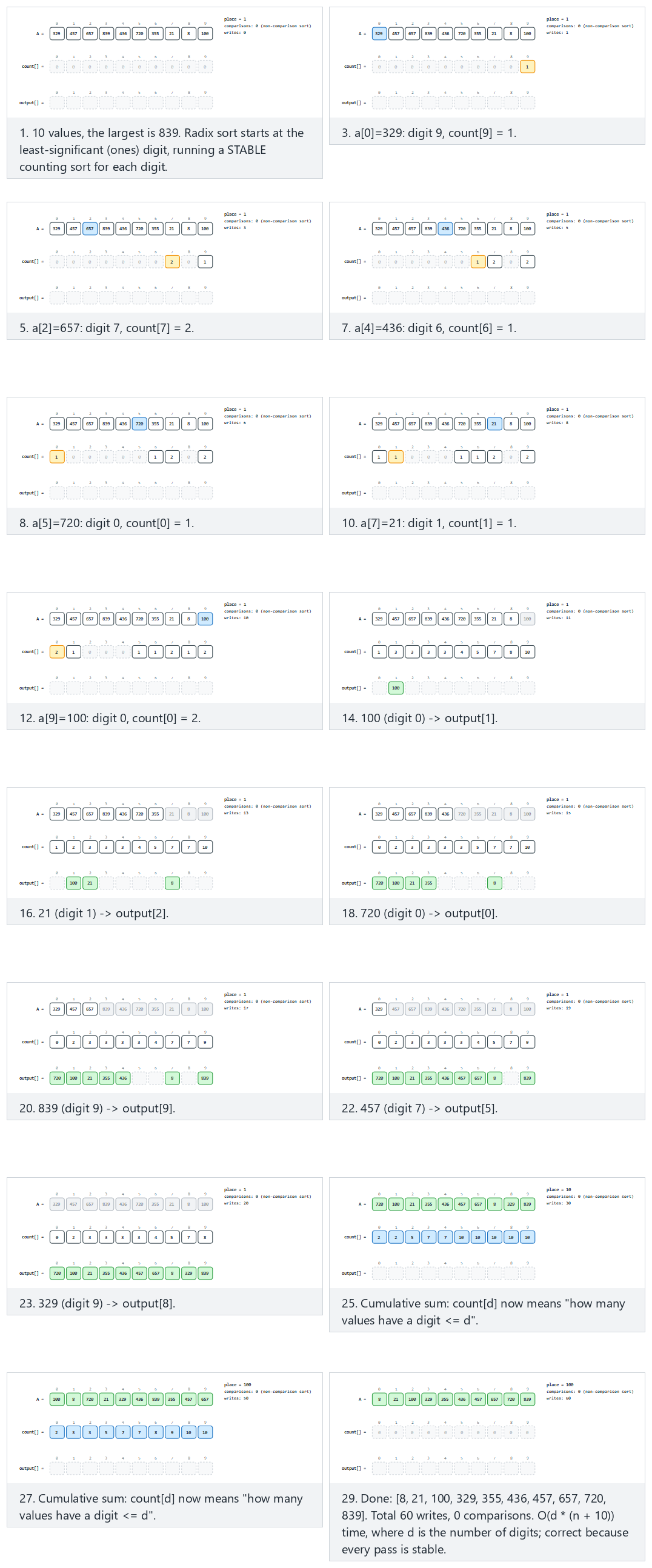
In the picker, also try all values single-digit — only one pass (the loop condition max_val / place > 0 naturally stops after the ones place once every value fits in one digit) and mixed digit lengths (shorter numbers behave exactly as if left-padded with invisible zero digits, since get_digit on a place beyond a value's own length simply returns 0), or press 🎲 for random data, or type your own array.
9.4 Try it
Full program: radix_sort_lsd.c / RadixSortLsd.java
/* Week 10 -- Sorting
 * Radix sort, least-significant-digit first (LSD): run a STABLE counting
 * sort on one decimal digit at a time, starting at the ones place, up to
 * the highest place any value needs. Always 10 buckets. Prints the array
 * after every digit pass. Zero comparisons; total writes are reported.
 * CEN207 Data Structures (formerly CE205)
 */
#include <stdio.h>

static int get_digit(int x, int place) { return (x / place) % 10; }

static void print_array(const int a[], int n) {
    printf("[");
    for (int i = 0; i < n; i++) printf("%d%s", a[i], i + 1 < n ? "," : "");
    printf("]\n");
}

void radix_sort_lsd(int a[], int n, int *writes) {
    if (n <= 0) return;               /* empty array: nothing to do, a[0] would be out of bounds */
    int max_val = a[0];
    for (int i = 1; i < n; i++) if (a[i] > max_val) max_val = a[i];

    for (int place = 1; max_val / place > 0; place *= 10) {
        int count[10] = {0};
        for (int i = 0; i < n; i++) { count[get_digit(a[i], place)]++; (*writes)++; }
        for (int d = 1; d < 10; d++) count[d] += count[d - 1];

        int output[64];
        for (int i = n - 1; i >= 0; i--) {
            int dgt = get_digit(a[i], place);
            output[count[dgt] - 1] = a[i];
            (*writes)++;
            count[dgt]--;
        }
        for (int i = 0; i < n; i++) a[i] = output[i];
        printf("  place=%-4d -> ", place);
        print_array(a, n);
    }
}

static void run_scenario(const char *label, int a[], int n) {
    printf("-- %s --\n", label);
    printf("before: ");
    print_array(a, n);
    int writes = 0;
    radix_sort_lsd(a, n, &writes);
    printf("after:  ");
    print_array(a, n);
    printf("total: 0 comparisons, %d writes\n\n", writes);
}

int main(void) {
    int normal[] = {329, 457, 657, 839, 436, 720, 355, 21, 8, 100};
    int hard[] = {5, 45, 802, 3, 66, 913, 27, 8, 150, 999, 12, 300, 4, 88};
    int already_sorted[] = {1, 12, 23, 34, 45, 56, 67, 78, 89, 90};
    int single_digit[] = {4, 2, 9, 1, 7, 3, 8, 0, 6, 5};

    run_scenario("normal: 10 values, up to 3 digits, 3 passes", normal, 10);
    run_scenario("hard: 14 values, mixed digit lengths", hard, 14);
    run_scenario("edge: already sorted -- every pass still runs", already_sorted, 10);
    run_scenario("edge: all single-digit values -- only one pass", single_digit, 10);

    return 0;
}
/* Week 10 -- Sorting
 * Radix sort, least-significant-digit first (LSD): run a STABLE counting
 * sort on one decimal digit at a time, starting at the ones place, up to
 * the highest place any value needs. Always 10 buckets. Prints the array
 * after every digit pass. Zero comparisons; total writes are reported.
 * CEN207 Data Structures (formerly CE205)
 */
public class RadixSortLsd {
    static int getDigit(int x, int place) { return (x / place) % 10; }

    static void printArray(int[] a) {
        StringBuilder sb = new StringBuilder("[");
        for (int i = 0; i < a.length; i++) { sb.append(a[i]); if (i + 1 < a.length) sb.append(','); }
        sb.append(']');
        System.out.println(sb);
    }

    static int radixSortLsd(int[] a, int n) {
        int writes = 0;
        if (n <= 0) return writes;    // empty array: nothing to do, a[0] would be out of bounds
        int maxVal = a[0];
        for (int i = 1; i < n; i++) if (a[i] > maxVal) maxVal = a[i];

        for (int place = 1; maxVal / place > 0; place *= 10) {
            int[] count = new int[10];
            for (int i = 0; i < n; i++) { count[getDigit(a[i], place)]++; writes++; }
            for (int d = 1; d < 10; d++) count[d] += count[d - 1];

            int[] output = new int[n];
            for (int i = n - 1; i >= 0; i--) {
                int dgt = getDigit(a[i], place);
                output[count[dgt] - 1] = a[i];
                writes++;
                count[dgt]--;
            }
            for (int i = 0; i < n; i++) a[i] = output[i];
            System.out.printf("  place=%-4d -> ", place);
            printArray(a);
        }
        return writes;
    }

    static void runScenario(String label, int[] a) {
        System.out.println("-- " + label + " --");
        System.out.print("before: ");
        printArray(a);
        int writes = radixSortLsd(a, a.length);
        System.out.print("after:  ");
        printArray(a);
        System.out.println("total: 0 comparisons, " + writes + " writes");
        System.out.println();
    }

    public static void main(String[] args) {
        int[] normal = {329, 457, 657, 839, 436, 720, 355, 21, 8, 100};
        int[] hard = {5, 45, 802, 3, 66, 913, 27, 8, 150, 999, 12, 300, 4, 88};
        int[] alreadySorted = {1, 12, 23, 34, 45, 56, 67, 78, 89, 90};
        int[] singleDigit = {4, 2, 9, 1, 7, 3, 8, 0, 6, 5};

        runScenario("normal: 10 values, up to 3 digits, 3 passes", normal);
        runScenario("hard: 14 values, mixed digit lengths", hard);
        runScenario("edge: already sorted -- every pass still runs", alreadySorted);
        runScenario("edge: all single-digit values -- only one pass", singleDigit);
    }
}
Try it
Expected output:
-- normal: 10 values, up to 3 digits, 3 passes --
before: [329,457,657,839,436,720,355,21,8,100]
  place=1    -> [720,100,21,355,436,457,657,8,329,839]
  place=10   -> [100,8,720,21,329,436,839,355,457,657]
  place=100  -> [8,21,100,329,355,436,457,657,720,839]
after:  [8,21,100,329,355,436,457,657,720,839]
total: 0 comparisons, 60 writes

-- hard: 14 values, mixed digit lengths --
before: [5,45,802,3,66,913,27,8,150,999,12,300,4,88]
  place=1    -> [150,300,802,12,3,913,4,5,45,66,27,8,88,999]
  place=10   -> [300,802,3,4,5,8,12,913,27,45,150,66,88,999]
  place=100  -> [3,4,5,8,12,27,45,66,88,150,300,802,913,999]
after:  [3,4,5,8,12,27,45,66,88,150,300,802,913,999]
total: 0 comparisons, 84 writes

-- edge: already sorted -- every pass still runs --
before: [1,12,23,34,45,56,67,78,89,90]
  place=1    -> [90,1,12,23,34,45,56,67,78,89]
  place=10   -> [1,12,23,34,45,56,67,78,89,90]
after:  [1,12,23,34,45,56,67,78,89,90]
total: 0 comparisons, 40 writes

-- edge: all single-digit values -- only one pass --
before: [4,2,9,1,7,3,8,0,6,5]
  place=1    -> [0,1,2,3,4,5,6,7,8,9]
after:  [0,1,2,3,4,5,6,7,8,9]
total: 0 comparisons, 20 writes
9.5 Complexity, mistakes, self-check
Complexity. O(d * (n + b)), where d is the number of digits the largest value has and b is the base (10 for decimal digits, so b is a small constant here). For fixed-width keys (32-bit integers, for instance, d is at most 10 in base 10, or a fixed 4 passes in base 65536) this is effectively O(n) — no log n factor anywhere, beating even the comparison-sort lower bound for the same reason counting sort does. Space: O(n + b), for output[] and count[]. Radix sort is stable, for the same reason as counting sort (section 8.5's self-check applies to every pass) — and that stability is not optional here, it is load- bearing: an unstable digit pass would scramble the ordering that earlier, less-significant passes already established, and the final result would not be correctly sorted at all.
Common mistakes
- Using an unstable sort for the per-digit pass. This is not merely a stability nicety here, unlike in most other contexts — radix sort's correctness depends on every pass being stable, because each pass relies on the previous pass's tie-breaking being preserved.
- Sorting from the most-significant digit instead of the least. An MSD-first radix sort exists too, but it needs a fundamentally different (recursive, per-bucket) structure to work correctly; naively running the LSD algorithm's logic starting from the highest digit does not produce a sorted array.
- Forgetting that shorter numbers act as if padded with leading zero digits.
get_digit(5, 100)correctly returns0(5 / 100 == 0,0 % 10 == 0) — no explicit padding logic is needed, but it is easy to assume, incorrectly, that a value needs special handling once the "current place" exceeds its own digit count.
Self-check: why LSD first, and not MSD first?
Explain, using the ideas from sections 8.5 and 9.2, why sorting by the least-significant digit first (and relying on each pass's stability) produces a correctly sorted array, while sorting by the most-significant digit first, using the exact same LSD algorithm unmodified, would not.
Answer. After the ones-place pass, the array is sorted by ones digit alone; after the tens-place pass, stability guarantees that any two values with the same tens digit keep the relative order the ones-place pass already gave them — so the array becomes correctly sorted by the two-digit number (tens, ones) together. This composes correctly all the way up: after the most significant digit's pass, ties broken by it were already correctly resolved by every less-significant digit in every earlier pass, so the whole array ends up sorted. Running the same algorithm starting from the most significant digit reverses this: the very first pass would group values by their leading digit, but within each group the remaining digits are still in their original, unsorted order — and no later pass (moving to less-significant digits) can fix that, because a stable pass on a less-significant digit does not know to keep each leading-digit group internally sorted by the digits already "settled." MSD-first radix sort is a real, different algorithm (used for variable-length keys like strings) that solves this by recursing separately into each bucket rather than doing flat passes — outside this week's scope.
10. Bucket sort
10.1 A question to start
Counting sort needs one count[] slot per possible value. Radix sort processes one digit at a time to keep that manageable for large integers. Bucket sort asks a related but different question: what if you do not even need exact counts up front — what if you can just throw each value into one of a small, fixed number of buckets based roughly on its magnitude, and then clean up each bucket (which, if the values are spread out reasonably evenly, will only ever hold a handful of elements) with a simple sort? This is the oldest and most general of this week's three non-comparison sorts — closer to "distribute into bins, then finish the job locally" than to counting sort's or radix sort's precise digit arithmetic — and it is usually presented as a natural generalization of counting sort rather than tied to one inventor or date.
10.2 The idea: distribute, sort small buckets, concatenate
For values known to lie in [0, max_val], divide that range into BUCKETS (this section uses 10) equal-sized intervals, and distribute every value into the bucket its interval covers — with max_val = 99 and 10 buckets, that interval size is exactly 10, so the bucket number is literally the tens digit. Sort each bucket individually (small buckets, so even plain insertion sort — section 4 — is cheap here). Concatenate the buckets in order, 0 through 9: since every value in bucket b is smaller than every value in bucket b+1 by construction (their intervals do not overlap), the concatenation is automatically fully sorted.
10.3 In memory, and the code
#define BUCKETS 10
#define MAX_N 20

void bucket_sort(int a[], int n, int max_val) {
    int bucket[BUCKETS][MAX_N];
    int bucket_len[BUCKETS] = {0};
    for (int i = 0; i < n; i++) {
        int b = (a[i] * BUCKETS) / (max_val + 1);   /* which bucket this value belongs to */
        bucket[b][bucket_len[b]++] = a[i];
    }
    int k = 0;
    for (int b = 0; b < BUCKETS; b++) {
        for (int x = 1; x < bucket_len[b]; x++) {          /* insertion sort within the bucket */
            int key = bucket[b][x], y = x - 1;
            while (y >= 0 && bucket[b][y] > key) { bucket[b][y + 1] = bucket[b][y]; y--; }
            bucket[b][y + 1] = key;
        }
        for (int i = 0; i < bucket_len[b]; i++) a[k++] = bucket[b][i];
    }
}
static final int BUCKETS = 10;
static final int MAX_N = 20;

void bucketSort(int[] a, int n, int maxVal) {
    int[][] bucket = new int[BUCKETS][MAX_N];
    int[] bucketLen = new int[BUCKETS];
    for (int i = 0; i < n; i++) {
        int b = (a[i] * BUCKETS) / (maxVal + 1);    // which bucket this value belongs to
        bucket[b][bucketLen[b]++] = a[i];
    }
    int k = 0;
    for (int b = 0; b < BUCKETS; b++) {
        for (int x = 1; x < bucketLen[b]; x++) {           // insertion sort within the bucket
            int key = bucket[b][x], y = x - 1;
            while (y >= 0 && bucket[b][y] > key) { bucket[b][y + 1] = bucket[b][y]; y--; }
            bucket[b][y + 1] = key;
        }
        for (int i = 0; i < bucketLen[b]; i++) a[k++] = bucket[b][i];
    }
}
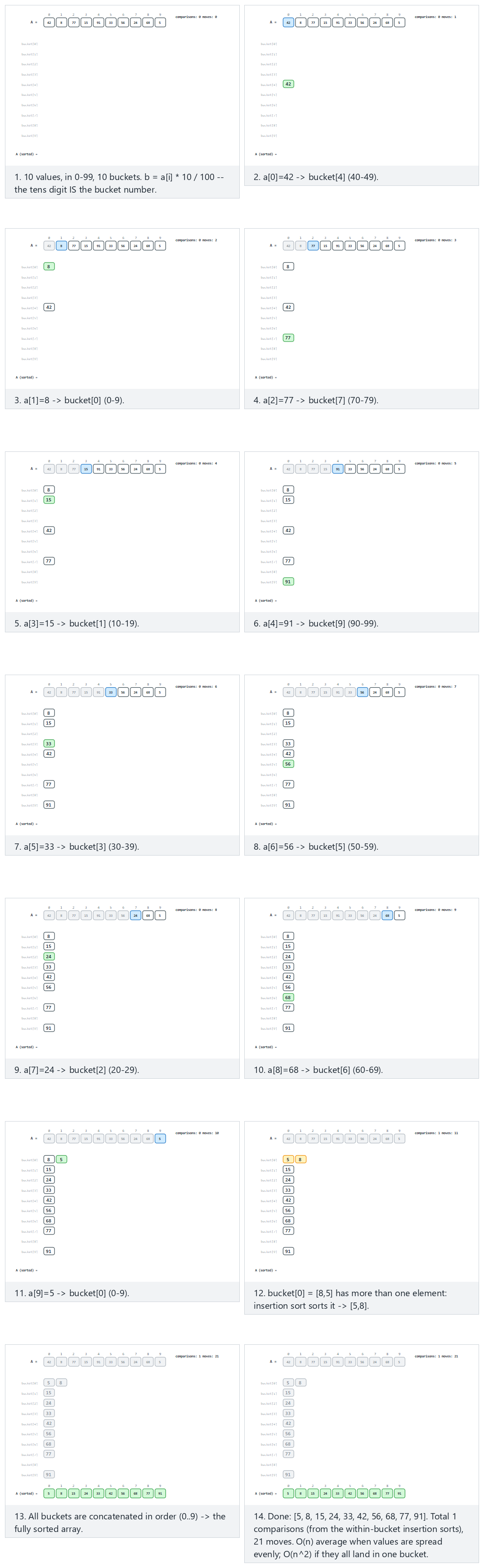
In the picker, also try all in one bucket — worst case, degrades to O(n²) (every one of the 10 values lands in bucket[4], so the "insertion sort within the bucket" step is really plain insertion sort on all n elements — bucket sort's average-case speed depends entirely on the input being roughly evenly spread), or press 🎲 for random data, or type your own array of values in 0..99.
10.4 Try it
Full program: bucket_sort.c / BucketSort.java
/* Week 10 -- Sorting
 * Bucket sort: for values in [0, 99], distribute into 10 buckets by the
 * tens digit, sort each bucket with insertion sort, then concatenate.
 * Prints the bucket contents and the final result; comparisons/moves are
 * counted (comparisons come from the within-bucket insertion sorts).
 * CEN207 Data Structures (formerly CE205)
 */
#include <stdio.h>

#define BUCKETS 10
#define MAX_N 20

static void print_array(const int a[], int n) {
    printf("[");
    for (int i = 0; i < n; i++) printf("%d%s", a[i], i + 1 < n ? "," : "");
    printf("]");
}

void bucket_sort(int a[], int n, int max_val, int *comparisons, int *moves) {
    int bucket[BUCKETS][MAX_N];
    int bucket_len[BUCKETS] = {0};
    for (int i = 0; i < n; i++) {
        int b = (a[i] * BUCKETS) / (max_val + 1);
        bucket[b][bucket_len[b]++] = a[i];
        (*moves)++;
    }
    int k = 0;
    for (int b = 0; b < BUCKETS; b++) {
        for (int x = 1; x < bucket_len[b]; x++) {
            int key = bucket[b][x], y = x - 1;
            while (y >= 0) {
                (*comparisons)++;
                if (bucket[b][y] <= key) break;
                bucket[b][y + 1] = bucket[b][y];
                (*moves)++;
                y--;
            }
            bucket[b][y + 1] = key;
        }
        if (bucket_len[b] > 0) {
            printf("  bucket[%d] (%d-%d) = ", b, 10 * b, 10 * b + 9);
            print_array(bucket[b], bucket_len[b]);
            printf("\n");
        }
        for (int i = 0; i < bucket_len[b]; i++) { a[k++] = bucket[b][i]; (*moves)++; }
    }
}

static void run_scenario(const char *label, int a[], int n) {
    printf("-- %s --\n", label);
    printf("before: ");
    print_array(a, n);
    printf("\n");
    int comparisons = 0, moves = 0;
    bucket_sort(a, n, 99, &comparisons, &moves);
    printf("after:  ");
    print_array(a, n);
    printf("\n");
    printf("total: %d comparisons, %d moves\n\n", comparisons, moves);
}

int main(void) {
    int normal[] = {42, 8, 77, 15, 91, 33, 56, 24, 68, 5};
    int hard[] = {42, 45, 8, 77, 71, 15, 91, 33, 38, 56, 24, 68, 5, 3};
    int same_bucket[] = {40, 41, 42, 43, 44, 45, 46, 47, 48, 49};
    int already_sorted[] = {2, 12, 22, 33, 44, 55, 66, 77, 88, 99};

    run_scenario("normal: 10 values, 0-99, spread well across the buckets", normal, 10);
    run_scenario("hard: 14 values, some buckets collide", hard, 14);
    run_scenario("edge: all in one bucket -- worst case, degrades to O(n^2)", same_bucket, 10);
    run_scenario("edge: already sorted", already_sorted, 10);

    return 0;
}
/* Week 10 -- Sorting
 * Bucket sort: for values in [0, 99], distribute into 10 buckets by the
 * tens digit, sort each bucket with insertion sort, then concatenate.
 * Prints the bucket contents and the final result; comparisons/moves are
 * counted (comparisons come from the within-bucket insertion sorts).
 * CEN207 Data Structures (formerly CE205)
 */
public class BucketSort {
    static final int BUCKETS = 10;
    static final int MAX_N = 20;
    static int comparisons, moves;

    static String arrStr(int[] a, int n) {
        StringBuilder sb = new StringBuilder("[");
        for (int i = 0; i < n; i++) { sb.append(a[i]); if (i + 1 < n) sb.append(','); }
        sb.append(']');
        return sb.toString();
    }

    static void bucketSort(int[] a, int n, int maxVal) {
        int[][] bucket = new int[BUCKETS][MAX_N];
        int[] bucketLen = new int[BUCKETS];
        for (int i = 0; i < n; i++) {
            int b = (a[i] * BUCKETS) / (maxVal + 1);
            bucket[b][bucketLen[b]++] = a[i];
            moves++;
        }
        int k = 0;
        for (int b = 0; b < BUCKETS; b++) {
            for (int x = 1; x < bucketLen[b]; x++) {
                int key = bucket[b][x], y = x - 1;
                while (y >= 0) {
                    comparisons++;
                    if (bucket[b][y] <= key) break;
                    bucket[b][y + 1] = bucket[b][y];
                    moves++;
                    y--;
                }
                bucket[b][y + 1] = key;
            }
            if (bucketLen[b] > 0) System.out.println("  bucket[" + b + "] (" + (10 * b) + "-" + (10 * b + 9) + ") = " + arrStr(bucket[b], bucketLen[b]));
            for (int i = 0; i < bucketLen[b]; i++) { a[k++] = bucket[b][i]; moves++; }
        }
    }

    static void runScenario(String label, int[] a) {
        System.out.println("-- " + label + " --");
        System.out.println("before: " + arrStr(a, a.length));
        comparisons = 0; moves = 0;
        bucketSort(a, a.length, 99);
        System.out.println("after:  " + arrStr(a, a.length));
        System.out.println("total: " + comparisons + " comparisons, " + moves + " moves");
        System.out.println();
    }

    public static void main(String[] args) {
        int[] normal = {42, 8, 77, 15, 91, 33, 56, 24, 68, 5};
        int[] hard = {42, 45, 8, 77, 71, 15, 91, 33, 38, 56, 24, 68, 5, 3};
        int[] sameBucket = {40, 41, 42, 43, 44, 45, 46, 47, 48, 49};
        int[] alreadySorted = {2, 12, 22, 33, 44, 55, 66, 77, 88, 99};

        runScenario("normal: 10 values, 0-99, spread well across the buckets", normal);
        runScenario("hard: 14 values, some buckets collide", hard);
        runScenario("edge: all in one bucket -- worst case, degrades to O(n^2)", sameBucket);
        runScenario("edge: already sorted", alreadySorted);
    }
}
Try it
Expected output:
-- normal: 10 values, 0-99, spread well across the buckets --
before: [42,8,77,15,91,33,56,24,68,5]
  bucket[0] (0-9) = [5,8]
  bucket[1] (10-19) = [15]
  bucket[2] (20-29) = [24]
  bucket[3] (30-39) = [33]
  bucket[4] (40-49) = [42]
  bucket[5] (50-59) = [56]
  bucket[6] (60-69) = [68]
  bucket[7] (70-79) = [77]
  bucket[9] (90-99) = [91]
after:  [5,8,15,24,33,42,56,68,77,91]
total: 1 comparisons, 21 moves

-- hard: 14 values, some buckets collide --
before: [42,45,8,77,71,15,91,33,38,56,24,68,5,3]
  bucket[0] (0-9) = [3,5,8]
  bucket[1] (10-19) = [15]
  bucket[2] (20-29) = [24]
  bucket[3] (30-39) = [33,38]
  bucket[4] (40-49) = [42,45]
  bucket[5] (50-59) = [56]
  bucket[6] (60-69) = [68]
  bucket[7] (70-79) = [71,77]
  bucket[9] (90-99) = [91]
after:  [3,5,8,15,24,33,38,42,45,56,68,71,77,91]
total: 6 comparisons, 32 moves

-- edge: all in one bucket -- worst case, degrades to O(n^2) --
before: [40,41,42,43,44,45,46,47,48,49]
  bucket[4] (40-49) = [40,41,42,43,44,45,46,47,48,49]
after:  [40,41,42,43,44,45,46,47,48,49]
total: 9 comparisons, 20 moves

-- edge: already sorted --
before: [2,12,22,33,44,55,66,77,88,99]
  bucket[0] (0-9) = [2]
  bucket[1] (10-19) = [12]
  bucket[2] (20-29) = [22]
  bucket[3] (30-39) = [33]
  bucket[4] (40-49) = [44]
  bucket[5] (50-59) = [55]
  bucket[6] (60-69) = [66]
  bucket[7] (70-79) = [77]
  bucket[8] (80-89) = [88]
  bucket[9] (90-99) = [99]
after:  [2,12,22,33,44,55,66,77,88,99]
total: 0 comparisons, 20 moves
10.5 Complexity, mistakes, self-check
Complexity. Average case O(n), when the n values are spread roughly evenly across the BUCKETS intervals: each bucket then holds about n / BUCKETS elements, and insertion-sorting a small, constant-size bucket costs O(1), so the total cost across all buckets is O(n). Worst case O(n^2), exactly when every value collides into one bucket (the "all in one bucket" example above: 9 comparisons for 10 values, which is already noticeably worse per-element than the well-spread example's 1 comparison for 10 values, and would grow quadratically for larger n) — at that point bucket sort has degraded into plain insertion sort on the whole array, with the bucket bookkeeping as pure overhead. Space: O(n + BUCKETS). Bucket sort is stable, provided the within-bucket sort used is itself stable (insertion sort is, as established in section 4.5) — values keep their relative order both within a bucket and across buckets, since buckets are concatenated in a fixed order that never mixes elements from different buckets.
Common mistakes
- Choosing a bucket count or range that does not match the data's actual distribution. Bucket sort's
O(n)average case is a promise about evenly spread data specifically — feeding it data that is naturally clustered (like the "all in one bucket" example, or real-world data with a skewed distribution) defeats the whole point, and there is no way to detect or fix this from inside the algorithm; it depends on choosing bucket boundaries that suit the actual data. - Using an unstable or expensive sort inside each bucket. Buckets are meant to be small, so insertion sort (section 4) is the natural choice — reaching for quick sort or another
O(n log n)sort here adds needless overhead for what should be a handful of elements, and using an unstable one throws away bucket sort's stability for no benefit. - Off-by-one in the bucket-index formula.
b = (a[i] * BUCKETS) / (max_val + 1)needs that+ 1in the denominator; without it, the maximum possible value (a[i] == max_val) computes to bucket indexBUCKETSitself — one past the last valid bucket, an out-of-bounds write.
Self-check: bucket sort versus counting sort
Both counting sort (section 8) and bucket sort distribute values by magnitude rather than comparing keys. Explain, in one or two sentences, the key structural difference between them, and why bucket sort needs an internal sort (like insertion sort) for each bucket while counting sort does not need anything similar for each count.
Answer. Counting sort keeps one exact count per individual value, so every value's final position is computed directly and precisely from the cumulative counts — there is nothing left to sort within a single value's group, since every occurrence of that value is interchangeable. Bucket sort keeps one bucket per range of values, so a bucket can hold several genuinely different values that still need to be placed in order relative to each other — hence the internal sort. This is exactly why bucket sort works for a wider variety of data (including, in its general form, floating-point values, which counting sort's per-value counting cannot handle directly) at the cost of needing that extra internal sorting step.
11. Stability, demonstrated
11.1 A question to start
Section 1.3 defined stability in words. Words are not proof. This section shows it happening on real data: the identical array of key+tag records, sorted by key with two different algorithms — one you already know is stable, one you already know is not — so you can watch the difference appear on screen instead of taking the definition on faith.
11.2 The idea: same input, two algorithms, compare the tag order
Every record is a (key, tag) pair, displayed as a short string like 5a — the number is the sort key, the letter is a stand-in for "which physical record this was" (imagine it as a row number, or a student's name, in a real dataset). Several records deliberately share the same key, so there is something for stability to be tested on. Row 1 runs insertion sort (section 4) — stable, because its shift condition is the strict a[j] > key, so an element only shifts past another with a strictly greater key: two records with equal keys are never swapped past each other. Row 2 runs selection sort (section 3) — not stable, because its swap moves the minimum directly from wherever it is found to position i, potentially jumping it past another record that happens to share its key and sits in between.
11.3 In memory, and the code
typedef struct { int key; char tag; } Rec;

void insertion_sort_stable(Rec a[], int n) {
    for (int i = 1; i < n; i++) {
        Rec key = a[i];
        int j = i - 1;
        while (j >= 0 && a[j].key > key.key) {   /* strict >: equal keys never cross */
            a[j + 1] = a[j];
            j--;
        }
        a[j + 1] = key;
    }
}

void selection_sort_unstable(Rec a[], int n) {
    for (int i = 0; i < n - 1; i++) {
        int min_idx = i;
        for (int j = i + 1; j < n; j++)
            if (a[j].key < a[min_idx].key) min_idx = j;
        if (min_idx != i) {
            Rec tmp = a[i]; a[i] = a[min_idx]; a[min_idx] = tmp;   /* can jump a tie out of order */
        }
    }
}
static class Rec { int key; char tag; Rec(int k, char t) { key = k; tag = t; } }

void insertionSortStable(Rec[] a, int n) {
    for (int i = 1; i < n; i++) {
        Rec key = a[i];
        int j = i - 1;
        while (j >= 0 && a[j].key > key.key) {   // strict >: equal keys never cross
            a[j + 1] = a[j];
            j--;
        }
        a[j + 1] = key;
    }
}

void selectionSortUnstable(Rec[] a, int n) {
    for (int i = 0; i < n - 1; i++) {
        int minIdx = i;
        for (int j = i + 1; j < n; j++)
            if (a[j].key < a[minIdx].key) minIdx = j;
        if (minIdx != i) {
            Rec tmp = a[i]; a[i] = a[minIdx]; a[minIdx] = tmp;    // can jump a tie out of order
        }
    }
}
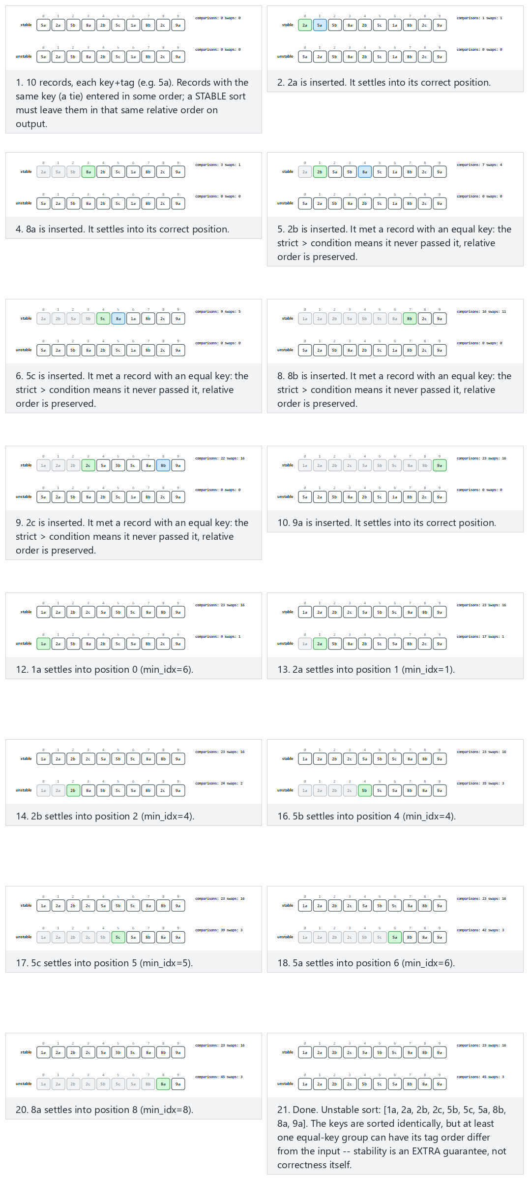
In the picker, the default normal example is the clearest demonstration: watch the 5a, 5b, 5c group specifically. In the picker, also try all keys equal — the whole array is one tie group (the most extreme case: a fully stable sort must reproduce the entire input order unchanged) or no ties at all — both sorts give the identical result (stability is invisible, and irrelevant, when there is nothing tied to preserve), or press 🎲 for random data, or type your own records as key+letter pairs (e.g. 5a 2a 5b).
11.4 Try it
Full program: stability_demo.c / StabilityDemo.java
/* Week 10 -- Sorting
 * Stability, demonstrated directly: the same key+tag records are sorted by
 * key with insertion sort (stable: strict `>` in the while condition means
 * equal keys never cross) and with selection sort (unstable: a long-range
 * swap can jump a record past another with an equal key). Prints both
 * results so the tag order for tied keys can be compared by eye.
 * CEN207 Data Structures (formerly CE205)
 */
#include <stdio.h>

typedef struct { int key; char tag; } Rec;

static void print_records(const Rec a[], int n) {
    printf("[");
    for (int i = 0; i < n; i++) printf("%d%c%s", a[i].key, a[i].tag, i + 1 < n ? " " : "");
    printf("]\n");
}

void insertion_sort_stable(Rec a[], int n) {
    for (int i = 1; i < n; i++) {
        Rec key = a[i];
        int j = i - 1;
        while (j >= 0 && a[j].key > key.key) {   /* strict >: equal keys never cross */
            a[j + 1] = a[j];
            j--;
        }
        a[j + 1] = key;
    }
}

void selection_sort_unstable(Rec a[], int n) {
    for (int i = 0; i < n - 1; i++) {
        int min_idx = i;
        for (int j = i + 1; j < n; j++)
            if (a[j].key < a[min_idx].key) min_idx = j;
        if (min_idx != i) {
            Rec tmp = a[i]; a[i] = a[min_idx]; a[min_idx] = tmp;   /* can jump a tie out of order */
        }
    }
}

static void run_scenario(const char *label, Rec src[], int n) {
    printf("-- %s --\n", label);
    printf("before:            ");
    print_records(src, n);

    Rec a1[16]; for (int i = 0; i < n; i++) a1[i] = src[i];
    insertion_sort_stable(a1, n);
    printf("stable (insert):   ");
    print_records(a1, n);

    Rec a2[16]; for (int i = 0; i < n; i++) a2[i] = src[i];
    selection_sort_unstable(a2, n);
    printf("unstable (select): ");
    print_records(a2, n);
    printf("\n");
}

int main(void) {
    Rec normal[] = {{5, 'a'}, {2, 'a'}, {5, 'b'}, {8, 'a'}, {2, 'b'}, {5, 'c'}, {1, 'a'}, {8, 'b'}, {2, 'c'}, {9, 'a'}};
    Rec all_equal[] = {{6, 'a'}, {6, 'b'}, {6, 'c'}, {6, 'd'}, {6, 'e'}, {6, 'f'}, {6, 'g'}, {6, 'h'}, {6, 'i'}, {6, 'j'}};
    Rec already_sorted[] = {{1, 'a'}, {2, 'a'}, {2, 'b'}, {3, 'a'}, {4, 'a'}, {4, 'b'}, {5, 'a'}, {6, 'a'}, {6, 'b'}, {7, 'a'}};
    Rec no_ties[] = {{9, 'a'}, {3, 'a'}, {7, 'a'}, {1, 'a'}, {5, 'a'}, {2, 'a'}, {8, 'a'}, {4, 'a'}, {6, 'a'}, {0, 'a'}};

    run_scenario("normal: 10 records, three groups of equal keys", normal, 10);
    run_scenario("edge: all keys equal -- the whole array is one tie group", all_equal, 10);
    run_scenario("edge: already-sorted keys, with ties present", already_sorted, 10);
    run_scenario("edge: no ties at all -- both sorts give the identical result", no_ties, 10);

    return 0;
}
/* Week 10 -- Sorting
 * Stability, demonstrated directly: the same key+tag records are sorted by
 * key with insertion sort (stable: strict > in the while condition means
 * equal keys never cross) and with selection sort (unstable: a long-range
 * swap can jump a record past another with an equal key). Prints both
 * results so the tag order for tied keys can be compared by eye.
 * CEN207 Data Structures (formerly CE205)
 */
public class StabilityDemo {
    static class Rec {
        int key; char tag;
        Rec(int key, char tag) { this.key = key; this.tag = tag; }
    }

    static String recordsStr(Rec[] a) {
        StringBuilder sb = new StringBuilder("[");
        for (int i = 0; i < a.length; i++) { sb.append(a[i].key).append(a[i].tag); if (i + 1 < a.length) sb.append(' '); }
        sb.append(']');
        return sb.toString();
    }

    static void insertionSortStable(Rec[] a) {
        int n = a.length;
        for (int i = 1; i < n; i++) {
            Rec key = a[i];
            int j = i - 1;
            while (j >= 0 && a[j].key > key.key) {   // strict >: equal keys never cross
                a[j + 1] = a[j];
                j--;
            }
            a[j + 1] = key;
        }
    }

    static void selectionSortUnstable(Rec[] a) {
        int n = a.length;
        for (int i = 0; i < n - 1; i++) {
            int minIdx = i;
            for (int j = i + 1; j < n; j++)
                if (a[j].key < a[minIdx].key) minIdx = j;
            if (minIdx != i) {
                Rec tmp = a[i]; a[i] = a[minIdx]; a[minIdx] = tmp;   // can jump a tie out of order
            }
        }
    }

    static Rec[] clone(Rec[] src) {
        Rec[] out = new Rec[src.length];
        for (int i = 0; i < src.length; i++) out[i] = new Rec(src[i].key, src[i].tag);
        return out;
    }

    static void runScenario(String label, Rec[] src) {
        System.out.println("-- " + label + " --");
        System.out.println("before:            " + recordsStr(src));

        Rec[] a1 = clone(src);
        insertionSortStable(a1);
        System.out.println("stable (insert):   " + recordsStr(a1));

        Rec[] a2 = clone(src);
        selectionSortUnstable(a2);
        System.out.println("unstable (select): " + recordsStr(a2));
        System.out.println();
    }

    public static void main(String[] args) {
        Rec[] normal = {new Rec(5, 'a'), new Rec(2, 'a'), new Rec(5, 'b'), new Rec(8, 'a'), new Rec(2, 'b'),
                         new Rec(5, 'c'), new Rec(1, 'a'), new Rec(8, 'b'), new Rec(2, 'c'), new Rec(9, 'a')};
        Rec[] allEqual = {new Rec(6, 'a'), new Rec(6, 'b'), new Rec(6, 'c'), new Rec(6, 'd'), new Rec(6, 'e'),
                           new Rec(6, 'f'), new Rec(6, 'g'), new Rec(6, 'h'), new Rec(6, 'i'), new Rec(6, 'j')};
        Rec[] alreadySorted = {new Rec(1, 'a'), new Rec(2, 'a'), new Rec(2, 'b'), new Rec(3, 'a'), new Rec(4, 'a'),
                                new Rec(4, 'b'), new Rec(5, 'a'), new Rec(6, 'a'), new Rec(6, 'b'), new Rec(7, 'a')};
        Rec[] noTies = {new Rec(9, 'a'), new Rec(3, 'a'), new Rec(7, 'a'), new Rec(1, 'a'), new Rec(5, 'a'),
                         new Rec(2, 'a'), new Rec(8, 'a'), new Rec(4, 'a'), new Rec(6, 'a'), new Rec(0, 'a')};

        runScenario("normal: 10 records, three groups of equal keys", normal);
        runScenario("edge: all keys equal -- the whole array is one tie group", allEqual);
        runScenario("edge: already-sorted keys, with ties present", alreadySorted);
        runScenario("edge: no ties at all -- both sorts give the identical result", noTies);
    }
}
Try it
Expected output:
-- normal: 10 records, three groups of equal keys --
before:            [5a 2a 5b 8a 2b 5c 1a 8b 2c 9a]
stable (insert):   [1a 2a 2b 2c 5a 5b 5c 8a 8b 9a]
unstable (select): [1a 2a 2b 2c 5b 5c 5a 8b 8a 9a]

-- edge: all keys equal -- the whole array is one tie group --
before:            [6a 6b 6c 6d 6e 6f 6g 6h 6i 6j]
stable (insert):   [6a 6b 6c 6d 6e 6f 6g 6h 6i 6j]
unstable (select): [6a 6b 6c 6d 6e 6f 6g 6h 6i 6j]

-- edge: already-sorted keys, with ties present --
before:            [1a 2a 2b 3a 4a 4b 5a 6a 6b 7a]
stable (insert):   [1a 2a 2b 3a 4a 4b 5a 6a 6b 7a]
unstable (select): [1a 2a 2b 3a 4a 4b 5a 6a 6b 7a]

-- edge: no ties at all -- both sorts give the identical result --
before:            [9a 3a 7a 1a 5a 2a 8a 4a 6a 0a]
stable (insert):   [0a 1a 2a 3a 4a 5a 6a 7a 8a 9a]
unstable (select): [0a 1a 2a 3a 4a 5a 6a 7a 8a 9a]
Look closely at the normal result: the stable sort's key-5 group reads 5a 5b 5c — exactly the input order. The unstable sort's key-5 group reads 5b 5c 5a — the 5a record, which appeared FIRST in the input, has been pushed to the END of its tie group. This is not a bug; it is selection sort's long-range swap doing exactly what section 3 described, on data specifically chosen to make the consequence visible. Notice, too, that the already-sorted example shows no difference at all between the two algorithms — when the input happens to already group equal keys together in a way neither algorithm's mechanics disturb, instability has nothing to act on.
11.5 Which of this week's algorithms are stable?
| Algorithm | Stable? | Why |
|---|---|---|
| Bubble sort (section 2) | Yes | swaps only on strict >; equal elements never cross |
| Selection sort (section 3) | No | the long-range swap can jump a tie out of order (demonstrated above) |
| Insertion sort (section 4) | Yes | shifts only on strict >; equal elements never cross |
| Shell sort (section 5) | No | gapped moves (gap > 1) can swap equal elements past each other |
| Merge sort (section 6) | Yes | the merge tie-break always prefers the left run first |
| Quick sort, Lomuto and Hoare (section 7) | No | both partitioning schemes swap across long distances with no regard for ties |
| Counting sort (section 8) | Yes | by construction, via the backward final placement scan |
| Radix sort, LSD (section 9) | Yes (required) | each digit pass must be stable for the whole algorithm to be correct |
| Bucket sort (section 10) | Yes, if the per-bucket sort is stable | insertion sort, used here, is stable |
Common mistakes
- Assuming an algorithm is stable "because it seems gentle" or unstable "because it seems aggressive." Stability is a precise structural property of the exact comparison/swap conditions used, not a vague impression — shell sort, for instance, looks like insertion sort but is not stable, because it moves elements
gappositions at a time instead of one at a time. - Caring about stability when it does not matter. If your sort key already uniquely identifies every record (no two records ever have equal keys), stability is unobservable — there is nothing left to preserve, and section 11.4's "no ties" example shows both a stable and an unstable sort producing an identical result.
- Needing stability and not checking for it. If you are sorting records by one field but need ties broken by a previous sort's order (a very common real pattern: sort by department, but within a department keep the existing name order), you must use a stable sort, or you must build the tie-break into your comparison explicitly (compare by the primary key, and on a tie, compare by the original index) — the table above tells you which of this week's algorithms you can rely on out of the box.
Self-check: forcing stability onto an unstable sort
Selection sort is not stable. Describe, in general terms (no code needed), one way to modify its comparison so that it becomes stable without changing which algorithm it fundamentally is.
Answer. Attach each element's original index to it (conceptually, sort pairs of (value, original index)), and change the comparison used to find the minimum so that on a tie in value, it prefers the element with the smaller original index. Selection sort will now always select the earliest-appearing among any tied minimum values, and since it still only performs a single swap per outer-loop iteration (moving that correctly-chosen minimum directly into place), the relative order of any group of equal values is preserved. This "compare by original index as a tie-break" technique works for making any unstable comparison-based sort stable, at the cost of the extra memory needed to track original indices — it is a general trick worth knowing, even though this week's specific algorithms do not need it applied to them (each one already is or is not stable by its own natural mechanics, as section 11.5 catalogs).
12. Comparing the algorithms, empirically
12.1 A question to start
Every section this week has claimed a Big-O complexity. Big-O describes growth rate, not an exact number — it deliberately hides the constant factors and lower-order terms that decide which of two O(n log n) algorithms is actually faster on a specific input of a specific size. The only way to settle "which sort actually wins on this data" is to run them and count. This section does exactly that: five algorithms (bubble, selection, insertion, merge, and quick with Lomuto partitioning), all sorting the identical array, with comparisons and writes counted through the same two counted primitives for every one of them, so the numbers are directly, fairly comparable.
12.2 In memory, and the code
sorting-comparison does not re-teach any single algorithm's mechanics — each already has its own dedicated animation earlier this week. Instead, every comparison and every array write funnels through two small counted primitives, so the tallies shown are a measurement, not an estimate:
int comparisons = 0, writes = 0;

int less(int a[], int x, int y) { comparisons++; return a[x] < a[y]; }
void write_at(int a[], int idx, int v) { writes++; a[idx] = v; }

/* every algorithm below is the SAME code from its own dedicated animation, except that
 * every comparison and every assignment into the array goes through less()/write_at() */
static int comparisons = 0, writes = 0;

static boolean less(int[] a, int x, int y) { comparisons++; return a[x] < a[y]; }
static void writeAt(int[] a, int idx, int v) { writes++; a[idx] = v; }

// every algorithm below is the SAME code from its own dedicated animation, except that
// every comparison and every assignment into the array goes through less()/writeAt()
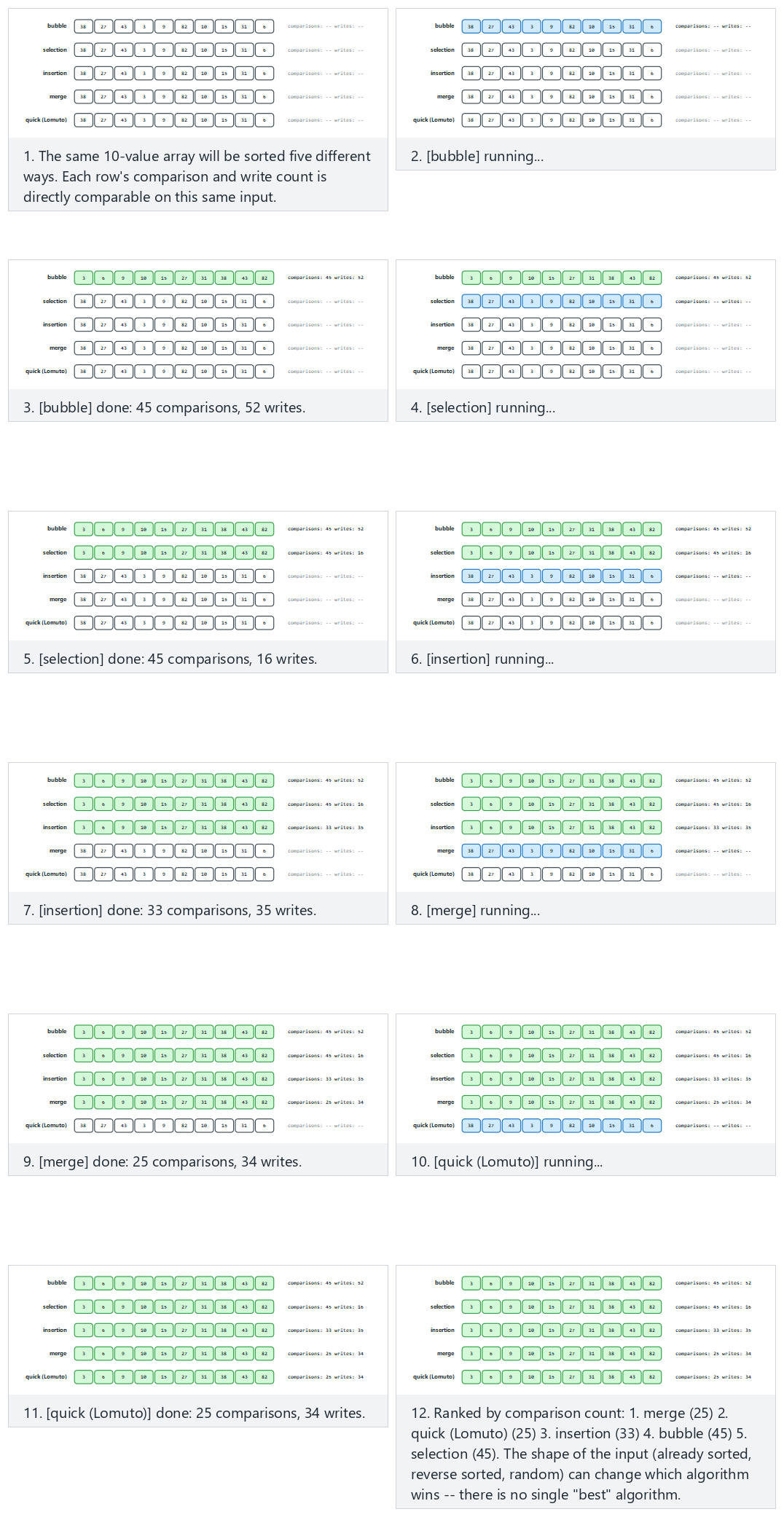
In the picker, the presets are the whole point: try already sorted and watch bubble sort win by a landslide (its early exit fires immediately) while quick sort (Lomuto) has its worst possible day on the exact same input — then try reverse sorted and watch quick sort's Lomuto partitioning hit its worst case again, this time alongside bubble sort also at its worst, both for the same underlying reason (a fixed, predictable comparison pattern that an adversarial input can exploit). Or press 🎲 for random data, or type your own array.
12.3 Try it
Full program: sorting_comparison.c / SortingComparison.java
/* Week 10 -- Sorting
 * Sorting comparison: the SAME input array is sorted five different ways
 * -- bubble, selection, insertion, merge (top-down), quick (Lomuto) -- and
 * each algorithm's comparisons/writes are reported on the identical input,
 * so the O(n^2) vs O(n log n) gap becomes an actual number.
 * CEN207 Data Structures (formerly CE205)
 */
#include <stdio.h>
#include <string.h>

static void print_array(const int a[], int n) {
    printf("[");
    for (int i = 0; i < n; i++) printf("%d%s", a[i], i + 1 < n ? "," : "");
    printf("]");
}

static void bubble(int a[], int n, int *comparisons, int *writes) {
    for (int pass = 0; pass < n - 1; pass++) {
        int swapped = 0;
        for (int i = 0; i < n - 1 - pass; i++) {
            (*comparisons)++;
            if (a[i] > a[i + 1]) { int t = a[i]; a[i] = a[i + 1]; a[i + 1] = t; *writes += 2; swapped = 1; }
        }
        if (!swapped) break;
    }
}

static void selection(int a[], int n, int *comparisons, int *writes) {
    for (int i = 0; i < n - 1; i++) {
        int m = i;
        for (int j = i + 1; j < n; j++) { (*comparisons)++; if (a[j] < a[m]) m = j; }
        if (m != i) { int t = a[i]; a[i] = a[m]; a[m] = t; *writes += 2; }
    }
}

static void insertion(int a[], int n, int *comparisons, int *writes) {
    for (int i = 1; i < n; i++) {
        int key = a[i], j = i - 1;
        while (j >= 0) {
            (*comparisons)++;
            if (a[j] <= key) break;
            a[j + 1] = a[j]; (*writes)++; j--;
        }
        a[j + 1] = key; (*writes)++;
    }
}

static void merge_range(int a[], int lo, int mid, int hi, int tmp[], int *comparisons, int *writes) {
    int i = lo, j = mid, k = lo;
    while (i < mid && j < hi) { (*comparisons)++; tmp[k++] = (a[i] <= a[j]) ? a[i++] : a[j++]; (*writes)++; }
    while (i < mid) { tmp[k++] = a[i++]; (*writes)++; }
    while (j < hi) { tmp[k++] = a[j++]; (*writes)++; }
    for (int x = lo; x < hi; x++) a[x] = tmp[x];
}
static void merge_sort_rec(int a[], int lo, int hi, int tmp[], int *comparisons, int *writes) {
    if (hi - lo <= 1) return;
    int mid = lo + (hi - lo) / 2;
    merge_sort_rec(a, lo, mid, tmp, comparisons, writes);
    merge_sort_rec(a, mid, hi, tmp, comparisons, writes);
    merge_range(a, lo, mid, hi, tmp, comparisons, writes);
}
static void merge_sort_top(int a[], int n, int *comparisons, int *writes) {
    int tmp[64];
    merge_sort_rec(a, 0, n, tmp, comparisons, writes);
}

static void quick_sort_rec(int a[], int lo, int hi, int *comparisons, int *writes) {
    if (lo >= hi) return;
    int pivot = a[hi], i = lo - 1;
    for (int j = lo; j < hi; j++) {
        (*comparisons)++;
        if (a[j] <= pivot) { i++; int t = a[i]; a[i] = a[j]; a[j] = t; *writes += 2; }
    }
    int t2 = a[i + 1]; a[i + 1] = a[hi]; a[hi] = t2; *writes += 2;
    int p = i + 1;
    quick_sort_rec(a, lo, p - 1, comparisons, writes);
    quick_sort_rec(a, p + 1, hi, comparisons, writes);
}
static void quick_sort_top(int a[], int n, int *comparisons, int *writes) { quick_sort_rec(a, 0, n - 1, comparisons, writes); }

typedef void (*SortFn)(int[], int, int *, int *);

static void run_one(const char *name, SortFn fn, const int src[], int n) {
    int a[32];
    memcpy(a, src, sizeof(int) * (size_t) n);
    int comparisons = 0, writes = 0;
    fn(a, n, &comparisons, &writes);
    printf("  %-10s comparisons=%-4d writes=%-4d -> ", name, comparisons, writes);
    print_array(a, n);
    printf("\n");
}

static void run_scenario(const char *label, const int a[], int n) {
    printf("-- %s --\n", label);
    printf("before: ");
    print_array(a, n);
    printf("\n");
    run_one("bubble", bubble, a, n);
    run_one("selection", selection, a, n);
    run_one("insertion", insertion, a, n);
    run_one("merge", merge_sort_top, a, n);
    run_one("quick", quick_sort_top, a, n);
    printf("\n");
}

int main(void) {
    int normal[] = {38, 27, 43, 3, 9, 82, 10, 15, 31, 6};
    int already_sorted[] = {1, 2, 3, 4, 5, 6, 7, 8, 9, 10, 11, 12};
    int reverse_sorted[] = {12, 11, 10, 9, 8, 7, 6, 5, 4, 3, 2, 1};
    int nearly_sorted[] = {1, 2, 3, 4, 9, 6, 7, 8, 5, 10, 11, 12};

    run_scenario("normal: 10 unordered values", normal, 10);
    run_scenario("edge: already sorted -- bubble wins via early exit, quick (Lomuto) has its worst day", already_sorted, 12);
    run_scenario("edge: reverse sorted -- both bubble and quick (Lomuto) hit their worst case", reverse_sorted, 12);
    run_scenario("edge: nearly sorted -- only two values are swapped", nearly_sorted, 12);

    return 0;
}
/* Week 10 -- Sorting
 * Sorting comparison: the SAME input array is sorted five different ways
 * -- bubble, selection, insertion, merge (top-down), quick (Lomuto) -- and
 * each algorithm's comparisons/writes are reported on the identical input,
 * so the O(n^2) vs O(n log n) gap becomes an actual number.
 * CEN207 Data Structures (formerly CE205)
 */
public class SortingComparison {
    interface SortFn { void sort(int[] a, int n); }

    static int comparisons, writes;

    static String arrStr(int[] a, int n) {
        StringBuilder sb = new StringBuilder("[");
        for (int i = 0; i < n; i++) { sb.append(a[i]); if (i + 1 < n) sb.append(','); }
        sb.append(']');
        return sb.toString();
    }

    static void bubble(int[] a, int n) {
        for (int pass = 0; pass < n - 1; pass++) {
            boolean swapped = false;
            for (int i = 0; i < n - 1 - pass; i++) {
                comparisons++;
                if (a[i] > a[i + 1]) { int t = a[i]; a[i] = a[i + 1]; a[i + 1] = t; writes += 2; swapped = true; }
            }
            if (!swapped) break;
        }
    }

    static void selection(int[] a, int n) {
        for (int i = 0; i < n - 1; i++) {
            int m = i;
            for (int j = i + 1; j < n; j++) { comparisons++; if (a[j] < a[m]) m = j; }
            if (m != i) { int t = a[i]; a[i] = a[m]; a[m] = t; writes += 2; }
        }
    }

    static void insertion(int[] a, int n) {
        for (int i = 1; i < n; i++) {
            int key = a[i], j = i - 1;
            while (j >= 0) {
                comparisons++;
                if (a[j] <= key) break;
                a[j + 1] = a[j]; writes++; j--;
            }
            a[j + 1] = key; writes++;
        }
    }

    static void mergeRange(int[] a, int lo, int mid, int hi, int[] tmp) {
        int i = lo, j = mid, k = lo;
        while (i < mid && j < hi) { comparisons++; tmp[k++] = (a[i] <= a[j]) ? a[i++] : a[j++]; writes++; }
        while (i < mid) { tmp[k++] = a[i++]; writes++; }
        while (j < hi) { tmp[k++] = a[j++]; writes++; }
        for (int x = lo; x < hi; x++) a[x] = tmp[x];
    }
    static void mergeSortRec(int[] a, int lo, int hi, int[] tmp) {
        if (hi - lo <= 1) return;
        int mid = lo + (hi - lo) / 2;
        mergeSortRec(a, lo, mid, tmp);
        mergeSortRec(a, mid, hi, tmp);
        mergeRange(a, lo, mid, hi, tmp);
    }
    static void mergeSortTop(int[] a, int n) { mergeSortRec(a, 0, n, new int[n]); }

    static void quickSortRec(int[] a, int lo, int hi) {
        if (lo >= hi) return;
        int pivot = a[hi], i = lo - 1;
        for (int j = lo; j < hi; j++) {
            comparisons++;
            if (a[j] <= pivot) { i++; int t = a[i]; a[i] = a[j]; a[j] = t; writes += 2; }
        }
        int t2 = a[i + 1]; a[i + 1] = a[hi]; a[hi] = t2; writes += 2;
        int p = i + 1;
        quickSortRec(a, lo, p - 1);
        quickSortRec(a, p + 1, hi);
    }
    static void quickSortTop(int[] a, int n) { quickSortRec(a, 0, n - 1); }

    static void runOne(String name, SortFn fn, int[] src, int n) {
        int[] a = new int[n];
        System.arraycopy(src, 0, a, 0, n);
        comparisons = 0; writes = 0;
        fn.sort(a, n);
        System.out.printf("  %-10s comparisons=%-4d writes=%-4d -> ", name, comparisons, writes);
        System.out.println(arrStr(a, n));
    }

    static void runScenario(String label, int[] a) {
        System.out.println("-- " + label + " --");
        System.out.println("before: " + arrStr(a, a.length));
        runOne("bubble", SortingComparison::bubble, a, a.length);
        runOne("selection", SortingComparison::selection, a, a.length);
        runOne("insertion", SortingComparison::insertion, a, a.length);
        runOne("merge", SortingComparison::mergeSortTop, a, a.length);
        runOne("quick", SortingComparison::quickSortTop, a, a.length);
        System.out.println();
    }

    public static void main(String[] args) {
        int[] normal = {38, 27, 43, 3, 9, 82, 10, 15, 31, 6};
        int[] alreadySorted = {1, 2, 3, 4, 5, 6, 7, 8, 9, 10, 11, 12};
        int[] reverseSorted = {12, 11, 10, 9, 8, 7, 6, 5, 4, 3, 2, 1};
        int[] nearlySorted = {1, 2, 3, 4, 9, 6, 7, 8, 5, 10, 11, 12};

        runScenario("normal: 10 unordered values", normal);
        runScenario("edge: already sorted -- bubble wins via early exit, quick (Lomuto) has its worst day", alreadySorted);
        runScenario("edge: reverse sorted -- both bubble and quick (Lomuto) hit their worst case", reverseSorted);
        runScenario("edge: nearly sorted -- only two values are swapped", nearlySorted);
    }
}
Try it
Expected output:
-- normal: 10 unordered values --
before: [38,27,43,3,9,82,10,15,31,6]
  bubble     comparisons=45   writes=52   -> [3,6,9,10,15,27,31,38,43,82]
  selection  comparisons=45   writes=16   -> [3,6,9,10,15,27,31,38,43,82]
  insertion  comparisons=33   writes=35   -> [3,6,9,10,15,27,31,38,43,82]
  merge      comparisons=25   writes=34   -> [3,6,9,10,15,27,31,38,43,82]
  quick      comparisons=25   writes=34   -> [3,6,9,10,15,27,31,38,43,82]

-- edge: already sorted -- bubble wins via early exit, quick (Lomuto) has its worst day --
before: [1,2,3,4,5,6,7,8,9,10,11,12]
  bubble     comparisons=11   writes=0    -> [1,2,3,4,5,6,7,8,9,10,11,12]
  selection  comparisons=66   writes=0    -> [1,2,3,4,5,6,7,8,9,10,11,12]
  insertion  comparisons=11   writes=11   -> [1,2,3,4,5,6,7,8,9,10,11,12]
  merge      comparisons=20   writes=44   -> [1,2,3,4,5,6,7,8,9,10,11,12]
  quick      comparisons=66   writes=154  -> [1,2,3,4,5,6,7,8,9,10,11,12]

-- edge: reverse sorted -- both bubble and quick (Lomuto) hit their worst case --
before: [12,11,10,9,8,7,6,5,4,3,2,1]
  bubble     comparisons=66   writes=132  -> [1,2,3,4,5,6,7,8,9,10,11,12]
  selection  comparisons=66   writes=12   -> [1,2,3,4,5,6,7,8,9,10,11,12]
  insertion  comparisons=66   writes=77   -> [1,2,3,4,5,6,7,8,9,10,11,12]
  merge      comparisons=24   writes=44   -> [1,2,3,4,5,6,7,8,9,10,11,12]
  quick      comparisons=66   writes=82   -> [1,2,3,4,5,6,7,8,9,10,11,12]

-- edge: nearly sorted -- only two values are swapped --
before: [1,2,3,4,9,6,7,8,5,10,11,12]
  bubble     comparisons=45   writes=14   -> [1,2,3,4,5,6,7,8,9,10,11,12]
  selection  comparisons=66   writes=2    -> [1,2,3,4,5,6,7,8,9,10,11,12]
  insertion  comparisons=18   writes=18   -> [1,2,3,4,5,6,7,8,9,10,11,12]
  merge      comparisons=24   writes=44   -> [1,2,3,4,5,6,7,8,9,10,11,12]
  quick      comparisons=50   writes=112  -> [1,2,3,4,5,6,7,8,9,10,11,12]
Four numbers tell the whole story of this week. On already-sorted input, bubble sort needs only 11 comparisons (its early exit, section 2) while quick sort (Lomuto) needs 66 — the exact worst case from section 7.5, on the exact same data. On nearly-sorted input (just two values swapped), insertion sort needs only 18 comparisons — close to its O(n) best case, since most elements are already in place (section 4.5's self-check) — while selection sort, which never benefits from partial ordering, still needs the full 66. There is no algorithm that wins every row of this table; which one you would actually pick depends entirely on what your input looks like, which is exactly section 13's subject.
13. Choosing a sorting algorithm
| Situation | Best choice | Why |
|---|---|---|
Tiny array (roughly n < 16), or a sub-array inside a bigger recursive sort | Insertion sort (section 4) | Lowest constant factor for small n; this is why real library sorts switch to it below a threshold |
| Data is already sorted, or very nearly so | Insertion sort, or bubble sort with its early exit | Both approach O(n) on nearly-sorted input; bubble sort's early exit and insertion sort's short shift chains both exploit it directly |
| Writes/swaps are expensive (large records, flash storage) but comparisons are cheap | Selection sort (section 3) | At most n-1 writes, guaranteed, regardless of input |
Need a guaranteed O(n log n) no matter what the input looks like, and extra memory is affordable | Merge sort (section 6) | The only sort this week with that guarantee in every case; also stable |
Need O(n log n) average performance, in place, extra memory is NOT affordable, and the input is not adversarial or already sorted | Quick sort with median-of-three (section 7.5) | Best real-world average performance and cache behavior; the median-of-three defense avoids the worst case on the common dangerous inputs (sorted/reverse-sorted) |
| Sorting must not use recursion (embedded systems, limited stack) | Merge sort, bottom-up (section 6.4), or heap sort (Week 4) | Both are iterative and O(n log n) with no call stack |
Keys are small non-negative integers, range not much larger than n | Counting sort (section 8) | O(n + k), beats the comparison lower bound entirely |
| Keys are larger integers (or fixed-length strings), too big a range for counting sort directly | Radix sort, LSD (section 9) | O(d * (n + b)), effectively O(n) for fixed-width keys |
| Keys are roughly uniformly spread over a known range | Bucket sort (section 10) | O(n) average when the spread assumption holds; degrades badly if it does not |
| Equal keys must keep their original relative order (a secondary sort key, or re-sorting after a previous stable sort) | Merge sort, insertion sort, bubble sort, counting sort, radix sort, or bucket sort with a stable inner sort | Section 11.5's table — never selection sort, shell sort, or quick sort unless you explicitly add a tie-break |
The single biggest decision is not "which sort is fastest in general" — section 12 showed there is no such thing, since the fastest algorithm changes depending on the input's shape. It is: what do you actually know about your data, and what do you actually need — a guarantee that holds no matter what (merge sort), the best average case in practice (quick sort), the fewest writes (selection sort), stability (several options), or a chance to sidestep comparison-sorting's O(n log n) lower bound entirely because your keys have special structure (counting, radix, or bucket sort). Knowing all eleven well enough to recognize which situation you are actually in — that is this week's real skill.
Summary
This week built a complete map of sorting: the simple, in-place O(n^2) family — bubble sort (adjacent swaps, an early exit that makes it O(n) best case), selection sort (find-the-minimum, at most n-1 swaps but always O(n^2) comparisons), insertion sort (grow a sorted prefix one key at a time, drawn with the "already sorted" brace / red key / shift-arrow model, O(n) best case on nearly-sorted data) — and shell sort, insertion sort sped up with a shrinking gap sequence. Then divide and conquer: merge sort, guaranteeing O(n log n) in every case at the cost of O(n) extra memory, in both its top-down (recursive, drawn as recursion-depth rows) and bottom-up (iterative, no recursion) forms; and quick sort, guaranteeing O(n log n) only on average but sorting in place, studied through both Lomuto (pivot = last, simpler) and Hoare (pivot = first, two inward scans, and the classic p vs. p - 1 recursion trap) partitioning, plus a direct numeric demonstration of how a naive fixed-corner pivot degrades to O(n^2) on sorted input and how median-of-three pivot selection avoids it. A fundamental theorem closed that half of the week: no comparison-based sort can ever guarantee better than O(n log n), because a decision tree distinguishing all n! orderings needs at least log2(n!) levels. The second half broke that bound entirely with three non-comparison sorts that never compare two keys against each other: counting sort (O(n + k), count occurrences, accumulate, place), radix sort (LSD-first, running a stable counting sort one decimal digit at a time — an idea traceable to Hollerith's 1890 census tabulating machines), and bucket sort (distribute into ranges, sort small buckets locally, concatenate). Along the way, stability — whether equal keys keep their input order — was defined, demonstrated directly on tagged data (insertion sort stable, selection sort not, on the identical input), and cataloged for all eleven algorithms; and five algorithms were raced against each other on identical inputs to show, with real numbers, that no single sort wins every situation — which is exactly why this course, and real software, keeps all of them in its toolbox.
Exercises
- Derive, from first principles, why bubble sort's early-exit optimization changes its best-case complexity from
O(n^2)toO(n), and construct a 10-element input (not simply "already sorted") on which the early exit fires after exactly the second pass, not the first. - Modify
selection_sort.cso that, instead of finding the minimum on each pass, it finds the minimum AND the maximum in a single pass (placing the minimum at the front and the maximum at the back, then shrinking the unsorted range from both ends). This is a real, named optimization ("cocktail" or "double-ended" selection sort) — trace by hand how many total passes it needs forn = 12compared to the original. - Using
insertion_sort.c's instrumented version, prove by construction that its total shift count for a reverse-sorted input of sizenis exactlyn(n-1)/2, and explain in one sentence why this is the same formula as bubble sort's worst-case swap count even though the two algorithms move data completely differently. - Trace
shell_sort.c's gap sequence by hand forn = 20(starting gap10, halving to1), listing every gap value used; then look up (you do not need to implement it) Hibbard's gap sequence2^k - 1for the samenand compare how many rounds each needs. - Using
merge_sort.c'smerge()function as a building block, describe (in words, or in code if you want the extra practice) how you would merge three already-sorted arrays into one, without simply merging them pairwise two at a time using the existing two-argumentmerge. What is the resulting time complexity in terms of the three arrays' combined sizen? - Prove the comparison-sorting lower bound yourself, following section 7.6's self-check: derive
log2(n!) = Omega(n log n)using Stirling's approximationn! ~ sqrt(2*pi*n) * (n/e)^n, showing the algebraic steps rather than quoting the result. quick_sort_worst_case.c'schoose_pivot_median3sorts three specific elements (a[lo],a[mid],a[hi]) partially in the course of finding their median. Trace by hand what final arrangement of those three positions the threeifstatements guarantee, and explain why that arrangement is not a full sort of all three (i.e., name a case where the three end up out of the fully sortedlo < mid < hiorder despite the median being correctly identified).- Using
counting_sort.c's "sparse range" scenario (maxVal = 15for only 10 values) as a starting point, compute the smallestn(number of values) at which you would judge that counting sort'sO(n + k)extra memory cost, fork = 1000, stops being worth it compared to simply usinginsertion_sort.cinstead — and justify your threshold with a rough operation-count comparison, not just intuition. radix_sort_lsd.cprocesses decimal digits (base 10). Rewrite (on paper; you do not need to run it) theget_digitfunction and the place-multiplication loop to process base 16 (hexadecimal) digits instead, using 16 buckets per pass — how many passes would a 32-bit unsigned integer need in base 16, compared to base 10?- Using
bucket_sort.c's bucket-index formulab = (a[i] * BUCKETS) / (max_val + 1), construct a 10-value input in the range[0, 99]that is deliberately spread as evenly as possible across all 10 buckets (at most one value per bucket beyond the minimum), and a second 10-value input that collides as many values as possible into a single bucket; run both through the program and report the comparison counts, confirming numerically which one is closer to bucket sort'sO(n)average case and which is closer to itsO(n^2)worst case.
Self-check quiz
1. Why does bubble sort's early-exit optimization not help selection sort at all, even though both grow a sorted region incrementally?
Bubble sort's early exit works because a pass making zero swaps is direct proof the whole array is already sorted — no further work could possibly be needed. Selection sort has no equivalent signal: finding the minimum of the remaining unsorted range fundamentally requires examining every element in that range, every single time, regardless of whether the array happens to already be sorted or not — there is no way to "notice" the array is sorted without doing the full scan that would notice it, so no early exit is possible.
2. Insertion sort and selection sort both grow a sorted region from the left. Explain the one-sentence mechanical difference that makes one stable and the other not.
Insertion sort's growing region is sorted because every new element is inserted into its correct spot inside it via single-step ADJACENT shifts, using a strict > comparison that never lets equal elements cross — so relative order among ties is preserved automatically. Selection sort's growing region is sorted because every new position is filled by a single LONG-RANGE swap that pulls the true minimum in from wherever it currently sits, which can relocate it past an equal-keyed element sitting in between, with no mechanism preventing that crossing.
3. Why is shell sort's worst-case complexity still O(n^2) with the simple n/2-halving gap sequence, despite it being empirically much faster than plain insertion sort?
The O(n^2) worst-case bound is a guarantee about the absolute worst possible input for that specific gap sequence — certain adversarial inputs exist that force even the large-gap passes to do nearly as much work as plain insertion sort would. In practice, on essentially all real and random inputs, the large early gaps move badly-placed elements most of the way home in very few shifts each (as section 5.5's self-check demonstrated numerically), which is why the empirical performance is far better than the worst-case bound would suggest — the gap sequence changes the AVERAGE and TYPICAL cost dramatically without changing the theoretical worst case for this particular sequence.
4. In merge sort, why must the auxiliary tmp array be at least as large as the range being merged, and why can the merge NOT be done directly within the original array with no extra space?
During a merge, the algorithm is simultaneously reading from both the left and right halves (via pointers i and j) while writing the merged, reordered result — and the position being written to (k) can still hold a value from either half that has not been read yet. Writing directly back into a[] risks overwriting a value before it has been compared and copied, corrupting the very data the merge still needs to read; the separate tmp array guarantees every write target is independent of every not-yet-read source, which is exactly the O(n) extra memory merge sort's O(n log n) guarantee costs.
5. Why does Hoare's partition scheme recurse on (lo, p) and (p + 1, hi), while Lomuto's recurses on (lo, p - 1) and (p + 1, hi) — same idea, different boundary?
Lomuto's partition guarantees, by construction, that the pivot itself ends up sitting exactly at the returned index p (its final swap explicitly puts it there) — so p is fully placed and correctly excluded from both recursive halves. Hoare's partition makes no such guarantee about where the pivot value itself ends up; it only guarantees that every index at or before the returned j holds a value <= pivot and every index after j holds a value >= pivot. Since the element at index p in Hoare's scheme might still need further sorting relative to its neighbors, excluding it (p - 1) as Lomuto does would incorrectly drop it from consideration — Hoare's correct recursive ranges must include p in the left half.
6. State the comparison-sorting lower bound in one sentence, and name the one property counting sort, radix sort, and bucket sort all share that lets them beat it.
No comparison-based sorting algorithm can guarantee fewer than O(n log n) comparisons in the worst case, because a binary decision tree distinguishing all n! possible input orderings needs at least log2(n!) levels. Counting sort, radix sort, and bucket sort all beat this bound by never comparing two keys against each other at all — they use the numeric VALUE of each key directly to compute its destination (a count, a digit, or a bucket index), which is a fundamentally different operation than a < or > comparison and is therefore simply not subject to the comparison-based lower bound.
7. Why is counting sort's O(n + k) guarantee not automatically an improvement over an O(n log n) comparison sort?
The bound is O(n + k), not O(n) — when k (the range of possible key values) is much larger than n (the number of elements actually being sorted), the k term dominates and can make counting sort far slower and far more memory-hungry than a comparison sort would have been, as section 8's "sparse range" example demonstrated directly (k = 15 for only n = 10 values already made the count[] array larger than the input itself). Counting sort is only a genuine win when k stays proportionate to, or smaller than, n.
8. Radix sort processes digits from least-significant to most-significant. Explain why every single pass must be stable for the final result to be correctly sorted, using the two-digit case as your example.
Consider two values that share the same tens digit but differ in their ones digit, versus two values that share the same ones digit but differ in their tens digit. After the ones-place pass, the array is correctly ordered by ones digit. When the tens-place pass then groups values by tens digit, a STABLE pass preserves whatever relative order those values already had from the ones-place pass — so within each tens-digit group, the values remain correctly ordered by ones digit too, giving a fully correct two-digit sort. If the tens-place pass were unstable, it could freely reorder values within a tens-digit group, destroying the ones-place ordering that pass had already correctly established, and the final result would not be sorted by the full two-digit value at all.
9. Bucket sort's average case is O(n). Describe the specific assumption about the input that this average-case analysis depends on, and what happens to bucket sort's performance when that assumption is violated.
The O(n) average case assumes the n input values are spread roughly EVENLY across the BUCKETS intervals, so that each bucket ends up holding only a small, roughly constant number of elements (around n / BUCKETS), making the per-bucket insertion sort cheap. When the assumption is violated — for instance, when the data is naturally clustered and many or all values land in the same bucket, as section 10's "all in one bucket" example demonstrated — bucket sort degrades to plain insertion sort on the whole array (or on whichever bucket absorbed most of the data), giving O(n^2) instead.
10. Given everything covered this week, in one or two sentences: why does this course teach eleven different sorting algorithms instead of just teaching the single fastest one?
Section 12 demonstrated with real, counted numbers that there is no single fastest algorithm across all inputs — bubble sort's early exit wins decisively on already-sorted data while being the worst choice on random data; quick sort wins on average for large random arrays but can degrade to the worst possible case on the exact kind of input (sorted or reverse-sorted) that is common in real systems; counting, radix, and bucket sort beat every comparison-based sort but only when the key structure actually supports them. Real software engineering requires recognizing which situation you are in — the shape of your data, your memory budget, whether you need a guarantee or just good average performance, whether you need stability — and section 13's decision table exists precisely because that answer is never the same algorithm twice.
Looking ahead
Weeks 7 and 8 were project demonstrations and a quiz, consolidating Weeks 1–6; this week, sorting, is the capstone of everything you have learned about arrays, complexity analysis, and recursion so far, and it feeds directly into the rest of the course. Week 11 moves to advanced tree structures, several of which depend directly on ideas from this week: balanced search trees maintain a sorted order incrementally as data arrives (rather than sorting a static array all at once, as every algorithm this week did), and you will see merge sort's divide-and-conquer pattern reappear in a tree-shaped form. Later weeks on file organization will return to sorting at a much larger scale — external sorting, where the data to be sorted is too large to fit in memory at all, and merge sort's ability to work from sorted "runs" (exactly the mechanism bottom-up merge sort used in section 6.4) becomes the foundation for sorting data that lives on disk.
References
- Course syllabus, Week 10:
CEN207-2026-2027-Guz-Izlence.en.md. - T. H. Cormen, C. E. Leiserson, R. L. Rivest, C. Stein. Introduction to Algorithms. MIT Press — the chapters on heapsort, quicksort (including the comparison-sorting lower bound proof), and sorting in linear time (counting sort, radix sort, bucket sort), in either the 3rd or 4th edition.
- D. E. Knuth. The Art of Computer Programming, Volume 3: Sorting and Searching, 2nd ed. Addison-Wesley, 1998 — the definitive historical and mathematical treatment of every algorithm in this chapter, including the early references to bubble sort and the analysis of shellsort's gap sequences.
- C. A. R. Hoare. "Quicksort." The Computer Journal, 5(1), 1962, pp. 10–16 — the original publication.
- D. L. Shell. "A High-Speed Sorting Procedure." Communications of the ACM, 2(7), 1959, pp. 30–32.
- R. Sedgewick, K. Wayne. Algorithms, 4th ed. Addison-Wesley, 2011 — the Sorting chapter (elementary sorts, mergesort, quicksort, priority queues) and its empirical comparison methodology, which this week's
sorting-comparisonanimation and section 12 follow in spirit. - williamfiset/Algorithms (https://github.com/williamfiset/Algorithms, MIT License) — Java reference implementations of comparison-based and non-comparison sorting algorithms.
- Programiz DSA (https://www.programiz.com/dsa) — step-by-step introductions to bubble, selection, insertion, shell, merge, quick, counting, radix, and bucket sort.
- Week 4 of this course — binary heaps and heap sort, the
O(n log n)in-place sort used throughout this week as a reference point.