Week 1 — Introduction to Data Structures
CEN207 Data Structures (formerly CE205) · Fall 2026–2027 · 18.09.2026
Lecture notes (PDF) Lecture notes (DOCX) Slides (PDF) Slides (PPTX) Slides (HTML, offline) Download all (ZIP) Open slides full screen
Click inside the slides and use the arrow keys; use the button at the bottom right of the slides, or the "Open slides full screen" link above, for full screen.
This week
Learning outcomes. This is the first week, so today is about building the foundation everything else in the course stands on. By the end of the week you will be able to say what a data structure is and why there is more than one kind; tell a linear structure from a non-linear one and place every structure you will meet this semester on one map; count the steps an algorithm takes and describe its growth with Big-O; explain what a pointer is in C and how a reference plays the same role in Java; draw the difference between the stack and the heap in memory, and what malloc/free and Java's new plus garbage collection each do about it; hand-encode a small record as TLV bytes, the same idea behind ASN.1's BER and PER; and, in a hands-on lab, compile, run and debug a C program with gcc, gdb and CMake. These outcomes map to LO.1 (explain the definitions, representations and basic operations of linear and non-linear data structures), LO.2 (analyze time and space complexity with Big-O), and LO.7 (select the data structures and algorithms best suited to a problem) of the course syllabus.
What you need already. Nothing from this course — it is week one. You do need the CEN107/CEN108 background listed on the prerequisites page: a working C toolchain, and enough C to read a loop and a function.
Time plan for a 3-hour session. Course plan and the map of the course (~15 min) · what a data structure is, linear vs non-linear (~25 min) · performance analysis and Big-O (~40 min) · short break · pointers, memory, stack and heap (~50 min) · ASN.1/TLV basics (~25 min) · hands-on C workshop lab (~25 min).
0. Before we start
0.1 Course plan and communication
The full weekly schedule, grading breakdown, textbooks and office-hours policy are in the syllabus; the term project you will build over the whole semester — first in C, then in Java — is described in the project guide; and the tools and background you are expected to already have are listed on the prerequisites page. Read all three before next week if you have not already. In class we will only touch the highlights: one project, two checkpoints (a midterm check in C, a final check in Java), weekly notes like this one in English and Turkish, and two quizzes (no separate homework). If anything in an older syllabus PDF ever looks out of date compared to what is said in class or in these notes, ask — do not guess.
0.2 The map of this week — and of the course
Data structures is a course about exactly two things: how to arrange data in memory, and how much that arrangement costs for the operations you actually need. Every week from here on introduces one more way to arrange data (linked lists, stacks and queues, trees, graphs, hash tables, files) and measures its cost with the tool you will learn today: Big-O. This week itself previews the whole map, then lays the two foundations — performance analysis, and memory (pointers, stack, heap) — that every later week assumes you already have.
flowchart TD
    W1["Week 1: foundations"]
    W1 --> DS["What is a data structure?"]
    W1 --> LN["Linear vs non-linear: the map of the course"]
    W1 --> BO["Performance analysis: Big-O"]
    W1 --> PT["Pointers and objects (C) / references (Java)"]
    W1 --> MEM["Memory: stack, heap, malloc/free, new + GC"]
    W1 --> TLV["ASN.1 / BER TLV / PER TLV basics"]
    W1 --> LAB["Hands-on lab: gcc, gdb, CMake"]
    LN --> LIN["Linear: arrays, linked lists, stacks, queues (Weeks 2-3)"]
    LN --> NONLIN["Non-linear: trees, graphs (Weeks 4-6)"]
    LN --> FLAT["Also linear, revisited later: hash tables, files (Weeks 7, 13-15)"]
    MEM --> W2PREVIEW["Preview: array vs linked layout (Week 2)"]
Every box under "Week 1: foundations" gets its own section below, most with a short step-by-step animation, a complete C and Java program, and a note on when things go wrong.
1. What is a data structure?
1.1 A question to start
Your phone's contacts app can find "Alice" among ten thousand names almost instantly, insert a new contact without re-sorting everything, and still list everyone alphabetically on demand. None of that is magic — it is a choice of how the names are arranged in memory. Arrange them differently (say, in the order you added them, with no structure at all) and the very same phone would need to scan every single name to find "Alice". The arrangement is the difference. That arrangement is what we call a data structure.
1.2 A short history
The term data structure itself became common in computer science through the 1960s, alongside the first systematic study of algorithms and their costs. Donald Knuth's The Art of Computer Programming, Volume 1: Fundamental Algorithms (1968) was the first major text to treat data structures — lists, stacks, trees — as objects of study in their own right, with their operations and costs analyzed side by side. A few years later, Barbara Liskov and Stephen Zilles (1974) gave the idea of an abstract data type — what a structure does, independent of how it is built — its modern, precise form, a distinction this course leans on constantly (you will meet it formally in Section 1.4 of Week 3, and informally starting today).
1.3 Intuition
Think of a data structure the way you think of furniture for storing physical things: a filing cabinet, a bookshelf sorted by author, a stack of trays on a desk, a phone book. Each one holds the same kind of content — papers, books, documents, names — but each one is good at different things. A stack of trays is fast to add to and take from at the top, terrible for finding something in the middle. A sorted bookshelf is fast to search, slow to insert into (you may have to shift many books to keep the order). There is no single "best" way to arrange things; there is only the best arrangement for what you are about to do with it.
A data structure is exactly this idea, made precise for a computer's memory: a way of organizing data so that certain operations — access an element, search for a value, insert a new one, delete one — can be done, and done at a known, analyzable cost.
1.4 Why there isn't just one
Every data structure makes trade-offs. The table below previews four operations that recur across this entire course; you will fill in the exact costs for each specific structure as you meet it in the coming weeks. For now, notice only the pattern: nothing is fast at everything.
| Operation | What it means | Why it isn't free |
|---|---|---|
| Access | Read the value at a given position | Some layouts compute a position directly (O(1)); others must walk from the start (O(n)) |
| Search | Find whether/where a value occurs | Unsorted data must be checked one by one; sorted data can be halved repeatedly (Week 3 previews this fully in Section 3 below) |
| Insert | Add a new value | Some layouts shift everything after the insertion point; others just relink a couple of pointers |
| Delete | Remove a value | Same trade-off as insert, mirrored |
Choosing a data structure is choosing which of these operations you need to be fast, because — as you will see concretely today and all semester — you cannot usually have all four be fast at once in the same structure.
2. Linear vs non-linear structures: the map of the course
2.1 A question to start
Take the last five songs you played and the org chart of a company. Both are collections of things, but they feel different to draw: the songs form a single line (song 1, then 2, then 3, ...), while the org chart branches (one CEO, several VPs, each with several reports). Is that difference just about drawing, or is it a real, structural fact about the data — one that changes what operations are cheap or expensive?
2.2 Definitions
A structure is linear when its elements form a sequence: every element (except the first) has exactly one element before it, and every element (except the last) has exactly one element after it. You can always ask "what comes next?" and get a single, unambiguous answer.
A structure is non-linear when an element can have more than one "next" (or more than one "previous"). A tree node can have several children; a graph node (often called a vertex) can connect to several others. There is no single "next" any more — traversing the structure means choosing which branch to follow.
2.3 The whole course, sorted onto this one line
Every structure you will meet this semester falls into one of these two families. Some, like hash tables and files, are still linear in how their slots are laid out, but solve a different problem (fast lookup by key, not by position) — we will point that out again when we get there.
| Family | Structure | When | Defining trade-off |
|---|---|---|---|
| Linear | Array | Week 2 | O(1) access by index; O(n) insert/delete in the middle |
| Linear | Linked list (singly, doubly, circular) | Week 2 | O(n) access; O(1) insert/delete once you are there |
| Linear | Stack (LIFO) | Week 3 | Touch one end only; every operation O(1) |
| Linear | Queue (FIFO) | Week 3 | Add at one end, remove at the other; every operation O(1) |
| Non-linear | Binary tree, heap | Week 4 | Each node has up to two children; O(log n) operations when balanced |
| Non-linear | Graph | Weeks 5–6 | Nodes connect to any number of others; models networks, maps, dependencies |
| Linear (by key) | Hash table | Week 7 | O(1) average access by key, not by position |
| Linear (on disk) | Sequential, direct and indexed files | Weeks 13–15 | The same trade-offs, now paid in disk I/O instead of memory access |
The mermaid map in Section 0.2 shows the same grouping visually. Keep coming back to it: every week adds exactly one row to this table, and every row is judged by the same measuring stick — the one you are about to learn.
Common mistakes
- Assuming "non-linear" means "disorganized". A tree and a graph are extremely structured — they simply allow more than one "next", which linear structures do not.
- Confusing "sorted" with "linear". A sorted array is linear (each element still has exactly one next); sorting is a property of the values, linearity is a property of the shape.
- Thinking a hash table or a file is an exception to everything you will learn about linear structures. Their slots are laid out linearly; only the access pattern (by key, via a computed position) is new. You will see this explicitly in Week 7.
Test yourself: linear vs non-linear
1. Is a stack of plates linear or non-linear? Why?
Linear: every plate (except the top one) has exactly one plate above it, and every plate (except the bottom one) has exactly one plate below it. There is a single, unambiguous "next".
2. Is a family tree linear or non-linear?
Non-linear: a parent can have several children, so there is more than one "next" from a given person.
3. Performance analysis: counting steps, not seconds
3.1 A question to start
You write a function that searches an array for a value. It works. Is it fast? Timing it on your laptop tells you about your laptop, today, for that one input size — a different machine, a bigger input, or a background process stealing CPU time can all change the number of seconds without the algorithm changing at all. What we actually want to know is a property of the algorithm itself: how does its work grow as the input grows? The tool for that question is Big-O, and the rest of this section builds it from scratch.
3.2 A short history
The notation predates computer science by decades: the German mathematician Paul Bachmann introduced the capital-O notation in 1894 to describe how closely one function approximates another, and Edmund Landau popularized and refined it in the early 1900s (it is still sometimes called a Landau symbol). Computer science adopted it to describe algorithm cost starting in the 1960s; Donald Knuth's widely read 1976 article "Big Omicron and Big Omega and Big Theta" (ACM SIGACT News) argued for, and helped standardize, exactly the O/Ω/Θ vocabulary this course uses.
3.3 Intuition: count the steps, not the seconds
Instead of a stopwatch, count how many times the algorithm does its basic unit of work — usually one comparison, one array access, or one arithmetic operation — as a function of the input size n. That count does not depend on the machine, the language, or how busy the computer is today; it depends only on the algorithm and n. Two searches over the same ten numbers make this concrete straightaway.
3.4 Linear search: try every box
Linear search starts at the front of the array and checks one element after another until it finds the target or runs out of elements. It needs no particular order in the data — it works on any array at all.
Play the animation to watch it count comparisons on an 11-element array, hunting for a value in the middle.
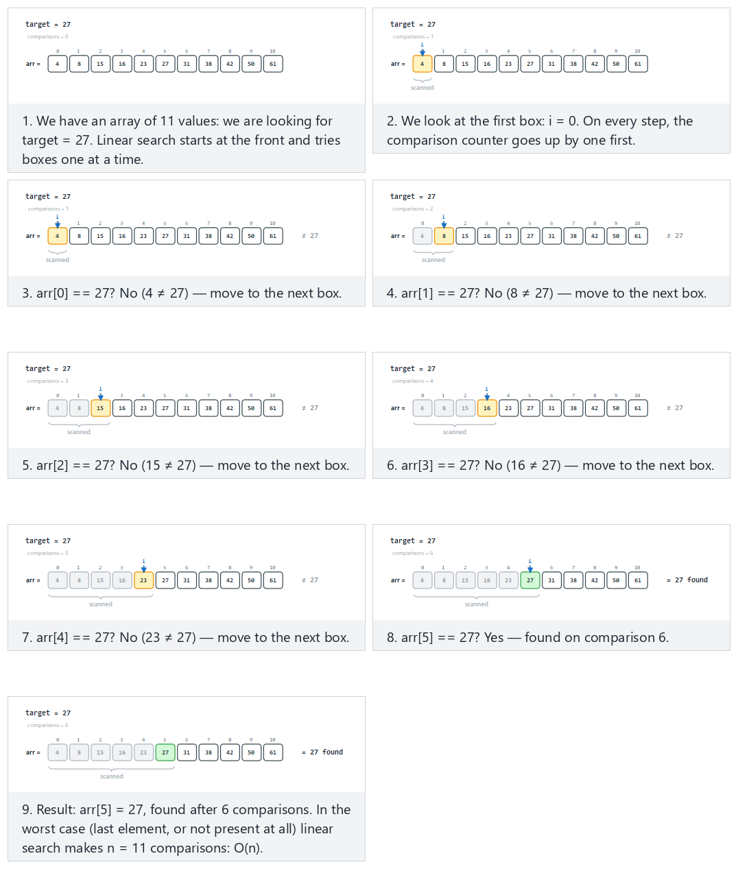
In the picker, also try 20 values, duplicate target, first match (hard) and the edge cases not found: target is not in the array, best case: target is in the first box (index 0), and one-element array — or press 🎲 for random data at four difficulty levels, or type your own array and target.
Full program: linear_search.c / LinearSearch.java
/* Week 1 -- Introduction to Data Structures
* Linear search: scan the array from the front, one comparison at a time.
* Runs the same normal / hard / edge-case scenarios as the linear-search animation.
* CEN207 Data Structures (CS50-style lecture notes)
*/
#include <stdio.h>
int linear_search(const int arr[], int n, int target, int *comparisons) {
    for (int i = 0; i < n; i++) {
        (*comparisons)++;
        if (arr[i] == target)
            return i;
    }
    return -1;
}
static void print_array(const int arr[], int n) {
printf("arr:");
for (int i = 0; i < n; i++)
printf(" %d", arr[i]);
printf(" (n = %d)\n", n);
}
static void run_scenario(const char *label, const int arr[], int n, int target) {
printf("-- %s --\n", label);
print_array(arr, n);
int comparisons = 0;
int index = linear_search(arr, n, target, &comparisons);
if (index >= 0)
printf("linear_search(target=%d) -> found at index %d, %d comparison%s\n\n",
target, index, comparisons, comparisons == 1 ? "" : "s");
else
printf("linear_search(target=%d) -> not found, %d comparisons\n\n", target, comparisons);
}
int main(void) {
/* normal: 11 values, target in the middle */
int normal[] = {4, 8, 15, 16, 23, 27, 31, 38, 42, 50, 61};
run_scenario("normal: 11 values, target in the middle", normal, 11, 27);
/* hard: 20 values, duplicate target, first match */
int hard[] = {12, 47, 3, 88, 25, 61, 9, 34, 77, 15, 52, 6, 41, 18, 63, 99, 5, 29, 99, 71};
run_scenario("hard: 20 values, duplicate target, first match", hard, 20, 99);
/* edge: not found -- target is not in the array */
int notFound[] = {2, 4, 6, 8, 10, 12, 14, 16, 18, 20};
run_scenario("edge: not found, target is not in the array", notFound, 10, 7);
/* edge: best case -- target is in the first box (index 0) */
int firstIndex[] = {5, 13, 21, 34, 42, 55, 67, 78, 89, 91};
run_scenario("edge: best case, target is in the first box (index 0)", firstIndex, 10, 5);
/* edge: one-element array */
int one[] = {42};
run_scenario("edge: one-element array", one, 1, 42);
return 0;
}
/* Week 1 -- Introduction to Data Structures
* Linear search: scan the array from the front, one comparison at a time.
* Runs the same normal / hard / edge-case scenarios as the linear-search animation.
* CEN207 Data Structures (CS50-style lecture notes)
*/
public class LinearSearch {
static int comparisons;
static int linearSearch(int[] arr, int target) {
    comparisons = 0;
    for (int i = 0; i < arr.length; i++) {
        comparisons++;
        if (arr[i] == target)
            return i;
    }
    return -1;
}
static void printArray(int[] arr) {
StringBuilder sb = new StringBuilder("arr:");
for (int v : arr) sb.append(' ').append(v);
sb.append(" (n = ").append(arr.length).append(')');
System.out.println(sb);
}
static void runScenario(String label, int[] arr, int target) {
System.out.println("-- " + label + " --");
printArray(arr);
int index = linearSearch(arr, target);
if (index >= 0)
System.out.println("linearSearch(target=" + target + ") -> found at index " + index
+ ", " + comparisons + " comparison" + (comparisons == 1 ? "" : "s"));
else
System.out.println("linearSearch(target=" + target + ") -> not found, "
+ comparisons + " comparisons");
System.out.println();
}
public static void main(String[] args) {
// normal: 11 values, target in the middle
int[] normal = {4, 8, 15, 16, 23, 27, 31, 38, 42, 50, 61};
runScenario("normal: 11 values, target in the middle", normal, 27);
// hard: 20 values, duplicate target, first match
int[] hard = {12, 47, 3, 88, 25, 61, 9, 34, 77, 15, 52, 6, 41, 18, 63, 99, 5, 29, 99, 71};
runScenario("hard: 20 values, duplicate target, first match", hard, 99);
// edge: not found -- target is not in the array
int[] notFound = {2, 4, 6, 8, 10, 12, 14, 16, 18, 20};
runScenario("edge: not found, target is not in the array", notFound, 7);
// edge: best case -- target is in the first box (index 0)
int[] firstIndex = {5, 13, 21, 34, 42, 55, 67, 78, 89, 91};
runScenario("edge: best case, target is in the first box (index 0)", firstIndex, 5);
// edge: one-element array
int[] one = {42};
runScenario("edge: one-element array", one, 42);
}
}
Full program: linear_search.c / LinearSearch.java
/* Week 1 -- Introduction to Data Structures
 * Linear search: scan the array from the front, one comparison at a time.
 * Runs the same normal / hard / edge-case scenarios as the linear-search animation.
 * CEN207 Data Structures (CS50-style lecture notes)
 */
#include <stdio.h>

int linear_search(const int arr[], int n, int target, int *comparisons) {
    for (int i = 0; i < n; i++) {
        (*comparisons)++;
        if (arr[i] == target)
            return i;
    }
    return -1;
}

static void print_array(const int arr[], int n) {
    printf("arr:");
    for (int i = 0; i < n; i++)
        printf(" %d", arr[i]);
    printf("  (n = %d)\n", n);
}

static void run_scenario(const char *label, const int arr[], int n, int target) {
    printf("-- %s --\n", label);
    print_array(arr, n);
    int comparisons = 0;
    int index = linear_search(arr, n, target, &comparisons);
    if (index >= 0)
        printf("linear_search(target=%d) -> found at index %d, %d comparison%s\n\n",
               target, index, comparisons, comparisons == 1 ? "" : "s");
    else
        printf("linear_search(target=%d) -> not found, %d comparisons\n\n", target, comparisons);
}

int main(void) {
    /* normal: 11 values, target in the middle */
    int normal[] = {4, 8, 15, 16, 23, 27, 31, 38, 42, 50, 61};
    run_scenario("normal: 11 values, target in the middle", normal, 11, 27);

    /* hard: 20 values, duplicate target, first match */
    int hard[] = {12, 47, 3, 88, 25, 61, 9, 34, 77, 15, 52, 6, 41, 18, 63, 99, 5, 29, 99, 71};
    run_scenario("hard: 20 values, duplicate target, first match", hard, 20, 99);

    /* edge: not found -- target is not in the array */
    int notFound[] = {2, 4, 6, 8, 10, 12, 14, 16, 18, 20};
    run_scenario("edge: not found, target is not in the array", notFound, 10, 7);

    /* edge: best case -- target is in the first box (index 0) */
    int firstIndex[] = {5, 13, 21, 34, 42, 55, 67, 78, 89, 91};
    run_scenario("edge: best case, target is in the first box (index 0)", firstIndex, 10, 5);

    /* edge: one-element array */
    int one[] = {42};
    run_scenario("edge: one-element array", one, 1, 42);

    return 0;
}
/* Week 1 -- Introduction to Data Structures
 * Linear search: scan the array from the front, one comparison at a time.
 * Runs the same normal / hard / edge-case scenarios as the linear-search animation.
 * CEN207 Data Structures (CS50-style lecture notes)
 */
public class LinearSearch {
    static int comparisons;

    static int linearSearch(int[] arr, int target) {
        comparisons = 0;
        for (int i = 0; i < arr.length; i++) {
            comparisons++;
            if (arr[i] == target)
                return i;
        }
        return -1;
    }

    static void printArray(int[] arr) {
        StringBuilder sb = new StringBuilder("arr:");
        for (int v : arr) sb.append(' ').append(v);
        sb.append("  (n = ").append(arr.length).append(')');
        System.out.println(sb);
    }

    static void runScenario(String label, int[] arr, int target) {
        System.out.println("-- " + label + " --");
        printArray(arr);
        int index = linearSearch(arr, target);
        if (index >= 0)
            System.out.println("linearSearch(target=" + target + ") -> found at index " + index
                    + ", " + comparisons + " comparison" + (comparisons == 1 ? "" : "s"));
        else
            System.out.println("linearSearch(target=" + target + ") -> not found, "
                    + comparisons + " comparisons");
        System.out.println();
    }

    public static void main(String[] args) {
        // normal: 11 values, target in the middle
        int[] normal = {4, 8, 15, 16, 23, 27, 31, 38, 42, 50, 61};
        runScenario("normal: 11 values, target in the middle", normal, 27);

        // hard: 20 values, duplicate target, first match
        int[] hard = {12, 47, 3, 88, 25, 61, 9, 34, 77, 15, 52, 6, 41, 18, 63, 99, 5, 29, 99, 71};
        runScenario("hard: 20 values, duplicate target, first match", hard, 99);

        // edge: not found -- target is not in the array
        int[] notFound = {2, 4, 6, 8, 10, 12, 14, 16, 18, 20};
        runScenario("edge: not found, target is not in the array", notFound, 7);

        // edge: best case -- target is in the first box (index 0)
        int[] firstIndex = {5, 13, 21, 34, 42, 55, 67, 78, 89, 91};
        runScenario("edge: best case, target is in the first box (index 0)", firstIndex, 5);

        // edge: one-element array
        int[] one = {42};
        runScenario("edge: one-element array", one, 42);
    }
}
Try it
Expected output:
-- normal: 11 values, target in the middle --
arr: 4 8 15 16 23 27 31 38 42 50 61  (n = 11)
linear_search(target=27) -> found at index 5, 6 comparisons

-- hard: 20 values, duplicate target, first match --
arr: 12 47 3 88 25 61 9 34 77 15 52 6 41 18 63 99 5 29 99 71  (n = 20)
linear_search(target=99) -> found at index 15, 16 comparisons

-- edge: not found, target is not in the array --
arr: 2 4 6 8 10 12 14 16 18 20  (n = 10)
linear_search(target=7) -> not found, 10 comparisons

-- edge: best case, target is in the first box (index 0) --
arr: 5 13 21 34 42 55 67 78 89 91  (n = 10)
linear_search(target=5) -> found at index 0, 1 comparison

-- edge: one-element array --
arr: 42  (n = 1)
linear_search(target=42) -> found at index 0, 1 comparison
Expected output:
-- normal: 11 values, target in the middle --
arr: 4 8 15 16 23 27 31 38 42 50 61  (n = 11)
linearSearch(target=27) -> found at index 5, 6 comparisons

-- hard: 20 values, duplicate target, first match --
arr: 12 47 3 88 25 61 9 34 77 15 52 6 41 18 63 99 5 29 99 71  (n = 20)
linearSearch(target=99) -> found at index 15, 16 comparisons

-- edge: not found, target is not in the array --
arr: 2 4 6 8 10 12 14 16 18 20  (n = 10)
linearSearch(target=7) -> not found, 10 comparisons

-- edge: best case, target is in the first box (index 0) --
arr: 5 13 21 34 42 55 67 78 89 91  (n = 10)
linearSearch(target=5) -> found at index 0, 1 comparison

-- edge: one-element array --
arr: 42  (n = 1)
linearSearch(target=42) -> found at index 0, 1 comparison
Eleven values or twenty, the shape stays the same: target = 27 sat at index 5, six comparisons in, and the hard scenario's duplicate 99 was found at its first occurrence (index 15, 16 comparisons), not its second. If the array had a million elements, the worst case would be a million comparisons. The cost grows directly with n — this is O(n), linear time.
3.5 Binary search: eliminate half the array every time
If the array is sorted, we can do far better. Check the middle element: if it is the target, we are done; if the target is smaller, it can only be in the left half, so throw away the right half (and vice versa). Repeat on the half that is left. This is binary search.
Play the animation on a 16-element sorted array, searching for 47.
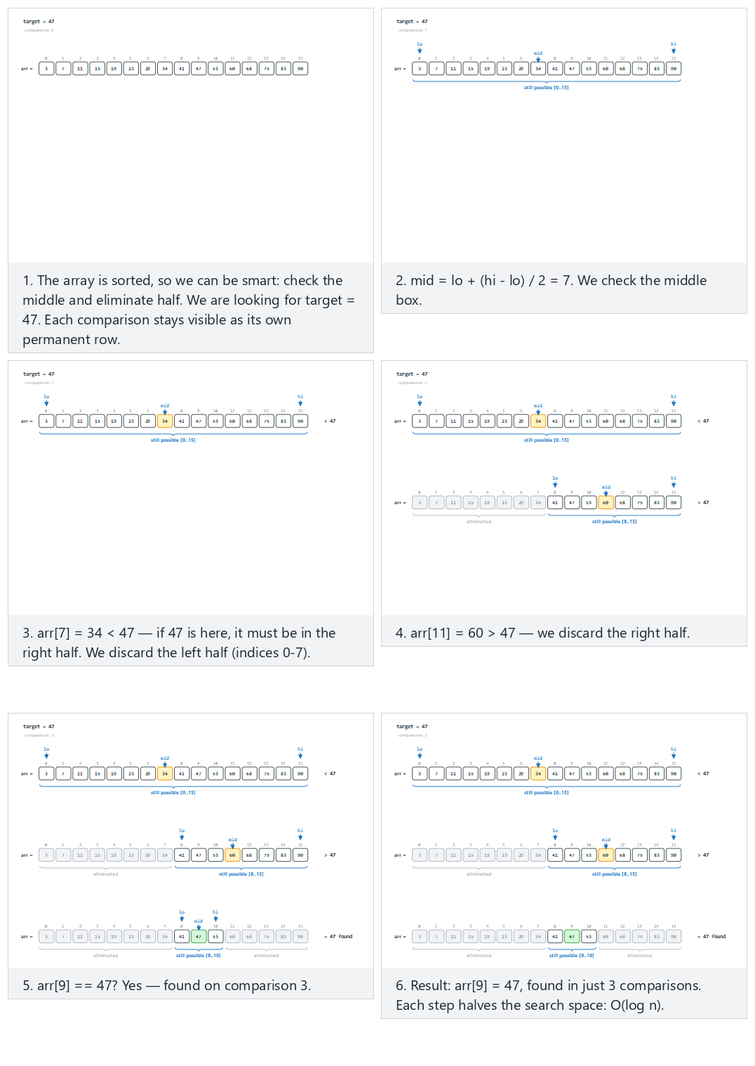
In the picker, also try 31 values, not found: lo > hi at the end (hard) and the edge cases target is smaller than every value, target is larger than every value, and searching among duplicate values — or press 🎲 for random data at four difficulty levels, or type your own sorted array and target.
static int binarySearch(int[] arr, int target) {
comparisons = 0;
int lo = 0, hi = arr.length - 1;
while (lo <= hi) {
int mid = lo + (hi - lo) / 2;
comparisons++;
if (arr[mid] == target)
return mid;
if (arr[mid] < target)
lo = mid + 1;
else
hi = mid - 1;
}
return -1;
}
The full class (code/week-01/java/BinarySearch.java) mirrors the C program's five scenarios exactly.
Full program: binary_search.c / BinarySearch.java
/* Week 1 -- Introduction to Data Structures
* Binary search: repeatedly halve the search range on a SORTED array.
* Runs the same normal / hard / edge-case scenarios as the binary-search animation.
* CEN207 Data Structures (CS50-style lecture notes)
*/
#include <stdio.h>
int binary_search(const int arr[], int n, int target, int *comparisons) {
    int lo = 0, hi = n - 1;
    while (lo <= hi) {
        int mid = lo + (hi - lo) / 2;
        (*comparisons)++;
        if (arr[mid] == target)
            return mid;
        if (arr[mid] < target)
            lo = mid + 1;
        else
            hi = mid - 1;
    }
    return -1;
}
static void print_array(const int arr[], int n) {
printf("arr:");
for (int i = 0; i < n; i++)
printf(" %d", arr[i]);
printf(" (n = %d)\n", n);
}
static void run_scenario(const char *label, const int arr[], int n, int target) {
printf("-- %s --\n", label);
print_array(arr, n);
int comparisons = 0;
int index = binary_search(arr, n, target, &comparisons);
if (index >= 0)
printf("binary_search(target=%d) -> found at index %d, %d comparison%s\n\n",
target, index, comparisons, comparisons == 1 ? "" : "s");
else
printf("binary_search(target=%d) -> not found, %d comparisons\n\n", target, comparisons);
}
int main(void) {
/* normal: 16 values, target found */
int normal[] = {3, 7, 11, 15, 19, 23, 29, 34, 41, 47, 53, 60, 68, 75, 83, 90};
run_scenario("normal: 16 values, target found", normal, 16, 47);
/* hard: 31 values, not found: lo > hi at the end */
int hard[] = {2, 6, 10, 14, 18, 22, 26, 30, 34, 38, 42, 46, 50, 54, 58, 62,
66, 70, 74, 78, 82, 86, 90, 94, 98, 102, 106, 110, 114, 118, 122};
run_scenario("hard: 31 values, not found (lo > hi at the end)", hard, 31, 5);
/* edge: target is smaller than every value */
int smallerThanAll[] = {10, 20, 30, 40, 50, 60, 70, 80, 90, 100};
run_scenario("edge: target is smaller than every value", smallerThanAll, 10, 1);
/* edge: target is larger than every value */
int largerThanAll[] = {15, 25, 35, 45, 55, 65, 75, 85, 95, 105};
run_scenario("edge: target is larger than every value", largerThanAll, 10, 999);
/* edge: searching among duplicate values */
int duplicates[] = {5, 5, 5, 10, 15, 20, 20, 25, 30, 35};
run_scenario("edge: searching among duplicate values", duplicates, 10, 20);
return 0;
}
/* Week 1 -- Introduction to Data Structures
* Binary search: repeatedly halve the search range on a SORTED array.
* Runs the same normal / hard / edge-case scenarios as the binary-search animation.
* CEN207 Data Structures (CS50-style lecture notes)
*/
public class BinarySearch {
static int comparisons;
static int binarySearch(int[] arr, int target) {
    comparisons = 0;
    int lo = 0, hi = arr.length - 1;
    while (lo <= hi) {
        int mid = lo + (hi - lo) / 2;
        comparisons++;
        if (arr[mid] == target)
            return mid;
        if (arr[mid] < target)
            lo = mid + 1;
        else
            hi = mid - 1;
    }
    return -1;
}
static void printArray(int[] arr) {
StringBuilder sb = new StringBuilder("arr:");
for (int v : arr) sb.append(' ').append(v);
sb.append(" (n = ").append(arr.length).append(')');
System.out.println(sb);
}
static void runScenario(String label, int[] arr, int target) {
System.out.println("-- " + label + " --");
printArray(arr);
int index = binarySearch(arr, target);
if (index >= 0)
System.out.println("binarySearch(target=" + target + ") -> found at index " + index
+ ", " + comparisons + " comparison" + (comparisons == 1 ? "" : "s"));
else
System.out.println("binarySearch(target=" + target + ") -> not found, "
+ comparisons + " comparisons");
System.out.println();
}
public static void main(String[] args) {
// normal: 16 values, target found
int[] normal = {3, 7, 11, 15, 19, 23, 29, 34, 41, 47, 53, 60, 68, 75, 83, 90};
runScenario("normal: 16 values, target found", normal, 47);
// hard: 31 values, not found: lo > hi at the end
int[] hard = {2, 6, 10, 14, 18, 22, 26, 30, 34, 38, 42, 46, 50, 54, 58, 62,
66, 70, 74, 78, 82, 86, 90, 94, 98, 102, 106, 110, 114, 118, 122};
runScenario("hard: 31 values, not found (lo > hi at the end)", hard, 5);
// edge: target is smaller than every value
int[] smallerThanAll = {10, 20, 30, 40, 50, 60, 70, 80, 90, 100};
runScenario("edge: target is smaller than every value", smallerThanAll, 1);
// edge: target is larger than every value
int[] largerThanAll = {15, 25, 35, 45, 55, 65, 75, 85, 95, 105};
runScenario("edge: target is larger than every value", largerThanAll, 999);
// edge: searching among duplicate values
int[] duplicates = {5, 5, 5, 10, 15, 20, 20, 25, 30, 35};
runScenario("edge: searching among duplicate values", duplicates, 20);
}
}
Full program: binary_search.c / BinarySearch.java
/* Week 1 -- Introduction to Data Structures
 * Binary search: repeatedly halve the search range on a SORTED array.
 * Runs the same normal / hard / edge-case scenarios as the binary-search animation.
 * CEN207 Data Structures (CS50-style lecture notes)
 */
#include <stdio.h>

int binary_search(const int arr[], int n, int target, int *comparisons) {
    int lo = 0, hi = n - 1;
    while (lo <= hi) {
        int mid = lo + (hi - lo) / 2;
        (*comparisons)++;
        if (arr[mid] == target)
            return mid;
        if (arr[mid] < target)
            lo = mid + 1;
        else
            hi = mid - 1;
    }
    return -1;
}

static void print_array(const int arr[], int n) {
    printf("arr:");
    for (int i = 0; i < n; i++)
        printf(" %d", arr[i]);
    printf("  (n = %d)\n", n);
}

static void run_scenario(const char *label, const int arr[], int n, int target) {
    printf("-- %s --\n", label);
    print_array(arr, n);
    int comparisons = 0;
    int index = binary_search(arr, n, target, &comparisons);
    if (index >= 0)
        printf("binary_search(target=%d) -> found at index %d, %d comparison%s\n\n",
               target, index, comparisons, comparisons == 1 ? "" : "s");
    else
        printf("binary_search(target=%d) -> not found, %d comparisons\n\n", target, comparisons);
}

int main(void) {
    /* normal: 16 values, target found */
    int normal[] = {3, 7, 11, 15, 19, 23, 29, 34, 41, 47, 53, 60, 68, 75, 83, 90};
    run_scenario("normal: 16 values, target found", normal, 16, 47);

    /* hard: 31 values, not found: lo > hi at the end */
    int hard[] = {2, 6, 10, 14, 18, 22, 26, 30, 34, 38, 42, 46, 50, 54, 58, 62,
                  66, 70, 74, 78, 82, 86, 90, 94, 98, 102, 106, 110, 114, 118, 122};
    run_scenario("hard: 31 values, not found (lo > hi at the end)", hard, 31, 5);

    /* edge: target is smaller than every value */
    int smallerThanAll[] = {10, 20, 30, 40, 50, 60, 70, 80, 90, 100};
    run_scenario("edge: target is smaller than every value", smallerThanAll, 10, 1);

    /* edge: target is larger than every value */
    int largerThanAll[] = {15, 25, 35, 45, 55, 65, 75, 85, 95, 105};
    run_scenario("edge: target is larger than every value", largerThanAll, 10, 999);

    /* edge: searching among duplicate values */
    int duplicates[] = {5, 5, 5, 10, 15, 20, 20, 25, 30, 35};
    run_scenario("edge: searching among duplicate values", duplicates, 10, 20);

    return 0;
}
/* Week 1 -- Introduction to Data Structures
 * Binary search: repeatedly halve the search range on a SORTED array.
 * Runs the same normal / hard / edge-case scenarios as the binary-search animation.
 * CEN207 Data Structures (CS50-style lecture notes)
 */
public class BinarySearch {
    static int comparisons;

    static int binarySearch(int[] arr, int target) {
        comparisons = 0;
        int lo = 0, hi = arr.length - 1;
        while (lo <= hi) {
            int mid = lo + (hi - lo) / 2;
            comparisons++;
            if (arr[mid] == target)
                return mid;
            if (arr[mid] < target)
                lo = mid + 1;
            else
                hi = mid - 1;
        }
        return -1;
    }

    static void printArray(int[] arr) {
        StringBuilder sb = new StringBuilder("arr:");
        for (int v : arr) sb.append(' ').append(v);
        sb.append("  (n = ").append(arr.length).append(')');
        System.out.println(sb);
    }

    static void runScenario(String label, int[] arr, int target) {
        System.out.println("-- " + label + " --");
        printArray(arr);
        int index = binarySearch(arr, target);
        if (index >= 0)
            System.out.println("binarySearch(target=" + target + ") -> found at index " + index
                    + ", " + comparisons + " comparison" + (comparisons == 1 ? "" : "s"));
        else
            System.out.println("binarySearch(target=" + target + ") -> not found, "
                    + comparisons + " comparisons");
        System.out.println();
    }

    public static void main(String[] args) {
        // normal: 16 values, target found
        int[] normal = {3, 7, 11, 15, 19, 23, 29, 34, 41, 47, 53, 60, 68, 75, 83, 90};
        runScenario("normal: 16 values, target found", normal, 47);

        // hard: 31 values, not found: lo > hi at the end
        int[] hard = {2, 6, 10, 14, 18, 22, 26, 30, 34, 38, 42, 46, 50, 54, 58, 62,
                      66, 70, 74, 78, 82, 86, 90, 94, 98, 102, 106, 110, 114, 118, 122};
        runScenario("hard: 31 values, not found (lo > hi at the end)", hard, 5);

        // edge: target is smaller than every value
        int[] smallerThanAll = {10, 20, 30, 40, 50, 60, 70, 80, 90, 100};
        runScenario("edge: target is smaller than every value", smallerThanAll, 1);

        // edge: target is larger than every value
        int[] largerThanAll = {15, 25, 35, 45, 55, 65, 75, 85, 95, 105};
        runScenario("edge: target is larger than every value", largerThanAll, 999);

        // edge: searching among duplicate values
        int[] duplicates = {5, 5, 5, 10, 15, 20, 20, 25, 30, 35};
        runScenario("edge: searching among duplicate values", duplicates, 20);
    }
}
Try it
Expected output:
-- normal: 16 values, target found --
arr: 3 7 11 15 19 23 29 34 41 47 53 60 68 75 83 90  (n = 16)
binary_search(target=47) -> found at index 9, 3 comparisons

-- hard: 31 values, not found (lo > hi at the end) --
arr: 2 6 10 14 18 22 26 30 34 38 42 46 50 54 58 62 66 70 74 78 82 86 90 94 98 102 106 110 114 118 122  (n = 31)
binary_search(target=5) -> not found, 5 comparisons

-- edge: target is smaller than every value --
arr: 10 20 30 40 50 60 70 80 90 100  (n = 10)
binary_search(target=1) -> not found, 3 comparisons

-- edge: target is larger than every value --
arr: 15 25 35 45 55 65 75 85 95 105  (n = 10)
binary_search(target=999) -> not found, 4 comparisons

-- edge: searching among duplicate values --
arr: 5 5 5 10 15 20 20 25 30 35  (n = 10)
binary_search(target=20) -> found at index 5, 3 comparisons
Expected output:
-- normal: 16 values, target found --
arr: 3 7 11 15 19 23 29 34 41 47 53 60 68 75 83 90  (n = 16)
binarySearch(target=47) -> found at index 9, 3 comparisons

-- hard: 31 values, not found (lo > hi at the end) --
arr: 2 6 10 14 18 22 26 30 34 38 42 46 50 54 58 62 66 70 74 78 82 86 90 94 98 102 106 110 114 118 122  (n = 31)
binarySearch(target=5) -> not found, 5 comparisons

-- edge: target is smaller than every value --
arr: 10 20 30 40 50 60 70 80 90 100  (n = 10)
binarySearch(target=1) -> not found, 3 comparisons

-- edge: target is larger than every value --
arr: 15 25 35 45 55 65 75 85 95 105  (n = 10)
binarySearch(target=999) -> not found, 4 comparisons

-- edge: searching among duplicate values --
arr: 5 5 5 10 15 20 20 25 30 35  (n = 10)
binarySearch(target=20) -> found at index 5, 3 comparisons
The same target = 47 that took linear search 6 comparisons (Section 3.4's normal scenario used a different array, but the shape holds generally) took binary search only 3 — and even the 31-element hard scenario, searching for a value not present at all, needed only 5. Every comparison throws away half of what is left, so the number of comparisons needed is the number of times you can halve n before reaching 1 — that is exactly log₂ n. This is O(log n), logarithmic time. The trade-off: binary search needs the array sorted first, and sorting itself costs more than one search (Week 9 covers sorting in depth).
3.6 The growth race: why the shape of the curve is what matters
O(n) and O(log n) are two points on a much larger scale. Watch five functions race as n doubles again and again, from 1 to 512: log₂n, n, n·log₂n (typical of the best sorting algorithms), n² (typical of the simplest ones, and of nested loops in general), and 2ⁿ (exponential — the Tower of Hanoi in Week 3).
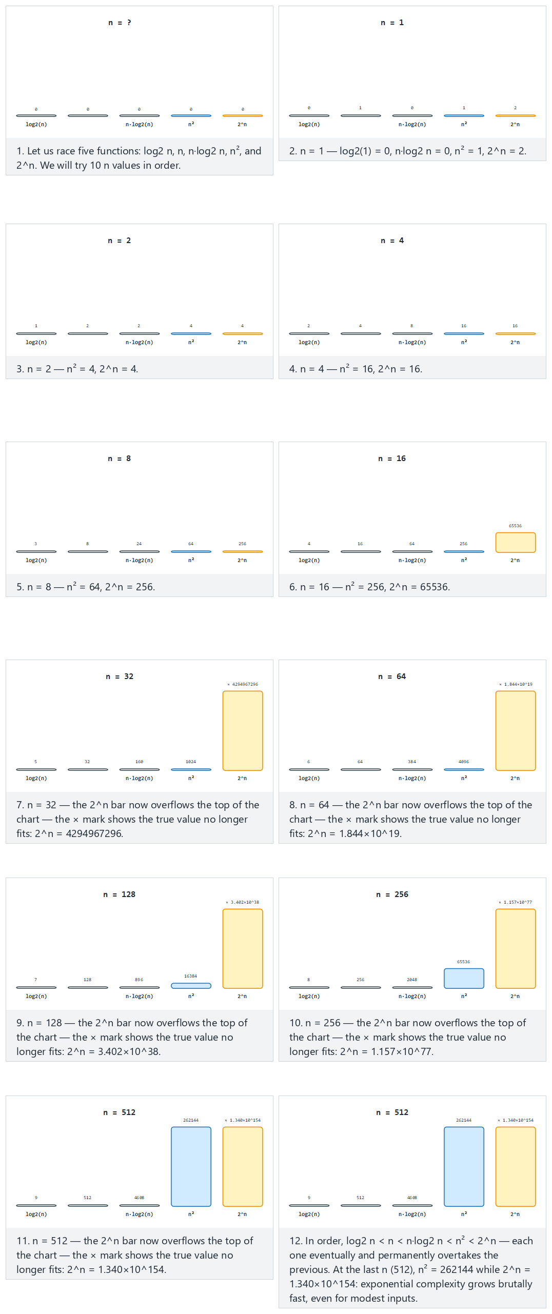
In the picker, also try doubling, longer: 1→4096 (hard) and the edge cases large n from the start: 2^n overflows on the very first step, a single value: n = 1, and an increasing sequence that is not a power of two — or press 🎲 for random data at four difficulty levels, or type your own list of n values.
The same five functions, computed for the animation's own n values instead of read off the bars. 2^n needs an exact, arbitrarily large integer once n passes a few dozen — Java's java.math.BigInteger gives that for free; C has no built-in big-integer type, so the C version below builds the exact decimal digit string itself, one doubling at a time (multiply every digit by 2, right to left, carrying into the next digit) — the standard grade-school-arithmetic trick, just automated.
/* out[] holds the decimal digits of 2^n, most significant digit first, NUL-terminated.
 * Doubling a decimal number is: multiply every digit by 2, right to left, carrying into the next digit. */
static void pow2_decimal(int n, char *out) {
    char digits[MAX_DIGITS];
    int len = 1;
    digits[0] = 1;   /* start at 2^0 = 1 */
    for (int step = 0; step < n; step++) {
        int carry = 0;
        for (int i = 0; i < len; i++) {
            int v = digits[i] * 2 + carry;
            digits[i] = (char) (v % 10);
            carry = v / 10;
        }
        if (carry) {
            digits[len] = (char) carry;
            len++;
        }
    }
    for (int i = 0; i < len; i++)
        out[i] = (char) ('0' + digits[len - 1 - i]);
    out[len] = '\0';
}
static void printRow(long n) {
    double log2n = Math.round(Math.log(n) / Math.log(2));
    double nlogn = Math.round(n * (Math.log(n) / Math.log(2)));
    long nsq = n * n;
    BigInteger pow2n = BigInteger.ONE.shiftLeft((int) n);   // exact, however large n is
    System.out.printf("n=%-6d log2(n)=%-4.0f n*log2(n)=%-8.0f n^2=%-9d 2^n=%s%n",
            n, log2n, nlogn, nsq, pow2n.toString());
}
The full class (code/week-01/java/GrowthTable.java) mirrors the C program's three scenarios exactly.
Full program: growth_table.c / GrowthTable.java
/* Week 1 -- Introduction to Data Structures
 * The growth race: for a list of n values, print log2(n), n, n*log2(n), n^2 and 2^n side by side.
 * 2^n is computed EXACTLY, as a decimal digit string built by repeated doubling (no library big-integer
 * type in C) so it can be compared byte for byte with Java's BigInteger version.
 * Runs the same normal / edge-case scenarios as the growth-race animation.
 * CEN207 Data Structures (CS50-style lecture notes)
 */
#include <math.h>
#include <stdio.h>
#include <string.h>

#define MAX_DIGITS 2000

/* out[] holds the decimal digits of 2^n, most significant digit first, NUL-terminated.
 * Doubling a decimal number is: multiply every digit by 2, right to left, carrying into the next digit. */
static void pow2_decimal(int n, char *out) {
    char digits[MAX_DIGITS];
    int len = 1;
    digits[0] = 1;   /* start at 2^0 = 1 */
    for (int step = 0; step < n; step++) {
        int carry = 0;
        for (int i = 0; i < len; i++) {
            int v = digits[i] * 2 + carry;
            digits[i] = (char) (v % 10);
            carry = v / 10;
        }
        if (carry) {
            digits[len] = (char) carry;
            len++;
        }
    }
    for (int i = 0; i < len; i++)
        out[i] = (char) ('0' + digits[len - 1 - i]);
    out[len] = '\0';
}

static void print_row(long n) {
    double log2n = round(log2((double) n));
    double nlogn = round((double) n * log2((double) n));
    long nsq = n * n;
    char pow2n[MAX_DIGITS];
    pow2_decimal((int) n, pow2n);
    printf("n=%-6ld log2(n)=%-4.0f n*log2(n)=%-8.0f n^2=%-9ld 2^n=%s\n", n, log2n, nlogn, nsq, pow2n);
}

static void run_scenario(const char *label, const long ns[], int count) {
    printf("-- %s --\n", label);
    for (int i = 0; i < count; i++)
        print_row(ns[i]);
    printf("\n");
}

int main(void) {
    /* normal: doubling, 1 -> 512 */
    long normal[] = {1, 2, 4, 8, 16, 32, 64, 128, 256, 512};
    run_scenario("normal: doubling, 1 -> 512", normal, 10);

    /* edge: a single value, n = 1 */
    long single[] = {1};
    run_scenario("edge: a single value, n = 1", single, 1);

    /* edge: an increasing sequence that is not a power of two */
    long nonPower[] = {1, 3, 5, 9, 14, 20, 27, 35, 44, 54};
    run_scenario("edge: an increasing sequence that is not a power of two", nonPower, 10);

    return 0;
}
/* Week 1 -- Introduction to Data Structures
 * The growth race: for a list of n values, print log2(n), n, n*log2(n), n^2 and 2^n side by side.
 * 2^n uses java.math.BigInteger, which gives EXACT arbitrary-precision integers out of the box --
 * unlike C, which has no built-in big-integer type (see growth_table.c's hand-rolled decimal doubling).
 * Runs the same normal / edge-case scenarios as the growth-race animation.
 * CEN207 Data Structures (CS50-style lecture notes)
 */
import java.math.BigInteger;

public class GrowthTable {
    static void printRow(long n) {
        double log2n = Math.round(Math.log(n) / Math.log(2));
        double nlogn = Math.round(n * (Math.log(n) / Math.log(2)));
        long nsq = n * n;
        BigInteger pow2n = BigInteger.ONE.shiftLeft((int) n);
        System.out.printf("n=%-6d log2(n)=%-4.0f n*log2(n)=%-8.0f n^2=%-9d 2^n=%s%n",
                n, log2n, nlogn, nsq, pow2n.toString());
    }

    static void runScenario(String label, long[] ns) {
        System.out.println("-- " + label + " --");
        for (long n : ns) printRow(n);
        System.out.println();
    }

    public static void main(String[] args) {
        // normal: doubling, 1 -> 512
        long[] normal = {1, 2, 4, 8, 16, 32, 64, 128, 256, 512};
        runScenario("normal: doubling, 1 -> 512", normal);

        // edge: a single value, n = 1
        long[] single = {1};
        runScenario("edge: a single value, n = 1", single);

        // edge: an increasing sequence that is not a power of two
        long[] nonPower = {1, 3, 5, 9, 14, 20, 27, 35, 44, 54};
        runScenario("edge: an increasing sequence that is not a power of two", nonPower);
    }
}
Full program: growth_table.c / GrowthTable.java
/* Week 1 -- Introduction to Data Structures
 * The growth race: for a list of n values, print log2(n), n, n*log2(n), n^2 and 2^n side by side.
 * 2^n is computed EXACTLY, as a decimal digit string built by repeated doubling (no library big-integer
 * type in C) so it can be compared byte for byte with Java's BigInteger version.
 * Runs the same normal / edge-case scenarios as the growth-race animation.
 * CEN207 Data Structures (CS50-style lecture notes)
 */
#include <math.h>
#include <stdio.h>
#include <string.h>

#define MAX_DIGITS 2000

/* out[] holds the decimal digits of 2^n, most significant digit first, NUL-terminated.
 * Doubling a decimal number is: multiply every digit by 2, right to left, carrying into the next digit. */
static void pow2_decimal(int n, char *out) {
    char digits[MAX_DIGITS];
    int len = 1;
    digits[0] = 1;   /* start at 2^0 = 1 */
    for (int step = 0; step < n; step++) {
        int carry = 0;
        for (int i = 0; i < len; i++) {
            int v = digits[i] * 2 + carry;
            digits[i] = (char) (v % 10);
            carry = v / 10;
        }
        if (carry) {
            digits[len] = (char) carry;
            len++;
        }
    }
    for (int i = 0; i < len; i++)
        out[i] = (char) ('0' + digits[len - 1 - i]);
    out[len] = '\0';
}

static void print_row(long n) {
    double log2n = round(log2((double) n));
    double nlogn = round((double) n * log2((double) n));
    long nsq = n * n;
    char pow2n[MAX_DIGITS];
    pow2_decimal((int) n, pow2n);
    printf("n=%-6ld log2(n)=%-4.0f n*log2(n)=%-8.0f n^2=%-9ld 2^n=%s\n", n, log2n, nlogn, nsq, pow2n);
}

static void run_scenario(const char *label, const long ns[], int count) {
    printf("-- %s --\n", label);
    for (int i = 0; i < count; i++)
        print_row(ns[i]);
    printf("\n");
}

int main(void) {
    /* normal: doubling, 1 -> 512 */
    long normal[] = {1, 2, 4, 8, 16, 32, 64, 128, 256, 512};
    run_scenario("normal: doubling, 1 -> 512", normal, 10);

    /* edge: a single value, n = 1 */
    long single[] = {1};
    run_scenario("edge: a single value, n = 1", single, 1);

    /* edge: an increasing sequence that is not a power of two */
    long nonPower[] = {1, 3, 5, 9, 14, 20, 27, 35, 44, 54};
    run_scenario("edge: an increasing sequence that is not a power of two", nonPower, 10);

    return 0;
}
/* Week 1 -- Introduction to Data Structures
 * The growth race: for a list of n values, print log2(n), n, n*log2(n), n^2 and 2^n side by side.
 * 2^n uses java.math.BigInteger, which gives EXACT arbitrary-precision integers out of the box --
 * unlike C, which has no built-in big-integer type (see growth_table.c's hand-rolled decimal doubling).
 * Runs the same normal / edge-case scenarios as the growth-race animation.
 * CEN207 Data Structures (CS50-style lecture notes)
 */
import java.math.BigInteger;

public class GrowthTable {
    static void printRow(long n) {
        double log2n = Math.round(Math.log(n) / Math.log(2));
        double nlogn = Math.round(n * (Math.log(n) / Math.log(2)));
        long nsq = n * n;
        BigInteger pow2n = BigInteger.ONE.shiftLeft((int) n);
        System.out.printf("n=%-6d log2(n)=%-4.0f n*log2(n)=%-8.0f n^2=%-9d 2^n=%s%n",
                n, log2n, nlogn, nsq, pow2n.toString());
    }

    static void runScenario(String label, long[] ns) {
        System.out.println("-- " + label + " --");
        for (long n : ns) printRow(n);
        System.out.println();
    }

    public static void main(String[] args) {
        // normal: doubling, 1 -> 512
        long[] normal = {1, 2, 4, 8, 16, 32, 64, 128, 256, 512};
        runScenario("normal: doubling, 1 -> 512", normal);

        // edge: a single value, n = 1
        long[] single = {1};
        runScenario("edge: a single value, n = 1", single);

        // edge: an increasing sequence that is not a power of two
        long[] nonPower = {1, 3, 5, 9, 14, 20, 27, 35, 44, 54};
        runScenario("edge: an increasing sequence that is not a power of two", nonPower);
    }
}
Try it
Expected output:
-- normal: doubling, 1 -> 512 --
n=1      log2(n)=0    n*log2(n)=0        n^2=1         2^n=2
n=2      log2(n)=1    n*log2(n)=2        n^2=4         2^n=4
n=4      log2(n)=2    n*log2(n)=8        n^2=16        2^n=16
n=8      log2(n)=3    n*log2(n)=24       n^2=64        2^n=256
n=16     log2(n)=4    n*log2(n)=64       n^2=256       2^n=65536
n=32     log2(n)=5    n*log2(n)=160      n^2=1024      2^n=4294967296
n=64     log2(n)=6    n*log2(n)=384      n^2=4096      2^n=18446744073709551616
n=128    log2(n)=7    n*log2(n)=896      n^2=16384     2^n=340282366920938463463374607431768211456
n=256    log2(n)=8    n*log2(n)=2048     n^2=65536     2^n=115792089237316195423570985008687907853269984665640564039457584007913129639936
n=512    log2(n)=9    n*log2(n)=4608     n^2=262144    2^n=13407807929942597099574024998205846127479365820592393377723561443721764030073546976801874298166903427690031858186486050853753882811946569946433649006084096

-- edge: a single value, n = 1 --
n=1      log2(n)=0    n*log2(n)=0        n^2=1         2^n=2

-- edge: an increasing sequence that is not a power of two --
n=1      log2(n)=0    n*log2(n)=0        n^2=1         2^n=2
n=3      log2(n)=2    n*log2(n)=5        n^2=9         2^n=8
n=5      log2(n)=2    n*log2(n)=12       n^2=25        2^n=32
n=9      log2(n)=3    n*log2(n)=29       n^2=81        2^n=512
n=14     log2(n)=4    n*log2(n)=53       n^2=196       2^n=16384
n=20     log2(n)=4    n*log2(n)=86       n^2=400       2^n=1048576
n=27     log2(n)=5    n*log2(n)=128      n^2=729       2^n=134217728
n=35     log2(n)=5    n*log2(n)=180      n^2=1225      2^n=34359738368
n=44     log2(n)=5    n*log2(n)=240      n^2=1936      2^n=17592186044416
n=54     log2(n)=6    n*log2(n)=311      n^2=2916      2^n=18014398509481984
At n = 512, n² is a modest 262144 but 2ⁿ is a number with 155 digits. An O(n²) algorithm and an O(2ⁿ) algorithm can both look instant on a toy input of a handful of elements and behave completely differently the moment n grows past a few dozen. This is the entire reason Big-O matters: it predicts what happens at the sizes you have not tested yet.
3.7 Big-O, precisely
Big-O describes an upper bound on how an algorithm's cost grows as n grows, ignoring constant factors and lower-order terms. Formally, f(n) is O(g(n)) if there exist constants c > 0 and n₀ such that f(n) ≤ c · g(n) for all n ≥ n₀ — in plain words, from some point on, f never grows faster than a constant multiple of g. In practice you rarely compute c and n₀; you count the steps, drop the constants and the smaller terms, and read off the dominant one:
| Steps counted | Dominant term | Big-O |
|---|---|---|
3n + 7 | n | O(n) |
n² + 2n + 1 | n² | O(n²) |
2·log₂n + 5 | log n | O(log n) |
100 (fixed, no matter what n is) | constant | O(1) |
From fastest-growing to slowest, the orders you will meet this semester are: O(1) < O(log n) < O(n) < O(n log n) < O(n²) < O(2ⁿ). You already met the first three today (constant-time array access from Week 1's own pointer arithmetic, O(log n) binary search, O(n) linear search); O(n log n) arrives with the good sorting algorithms in Week 9, O(2ⁿ) with the Tower of Hanoi in Week 3.
Let's build one of these formulas by hand instead of taking the table on faith. A nested loop — a loop inside another loop — is the classic source of an n² term: for every one of the n outer iterations, the inner loop runs all n of its own iterations.
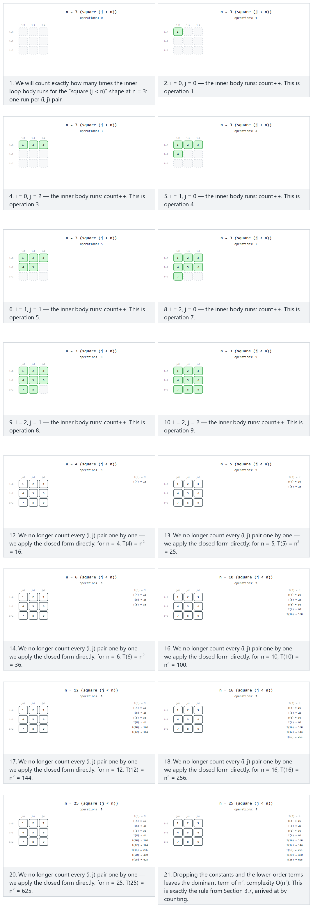
In the picker, also try triangle loop, n = 4 in detail, then 10 more n values (hard) and the edge cases halving loop, n = 1: zero executions and square loop, n = 2 in detail, Fibonacci-spaced n values — or press 🎲 for random data at four difficulty levels, or type your own shape and n values.
static long tSquare(int n) {
long count = 0;
for (int i = 0; i < n; i++) {
for (int j = 0; j < n; j++) {
count++;
operations++;
}
}
return count;
}
The full class (code/week-01/java/NestedLoopCounting.java) also has tTriangle (j < i) and tHalving (j *= 2), and mirrors the C program's four scenarios exactly.
Full program: nested_loop_counting.c / NestedLoopCounting.java
/* Week 1 -- Introduction to Data Structures
* Count the operations of a nested loop to build T(n) by hand, for three loop shapes:
* square (j < n), triangle (j < i), and halving (j *= 2).
* Runs the same normal / hard / edge-case scenarios as the nested-loop-counting animation.
* CEN207 Data Structures (CS50-style lecture notes)
*/
#include <stdio.h>
long t_square(int n, long *operations) {
    long count = 0;
    for (int i = 0; i < n; i++) {
        for (int j = 0; j < n; j++) {
            count++;
            (*operations)++;
        }
    }
    return count;
}
long t_triangle(int n, long *operations) {
long count = 0;
for (int i = 0; i < n; i++) {
for (int j = 0; j < i; j++) {
count++;
(*operations)++;
}
}
return count;
}
long t_halving(int n, long *operations) {
long count = 0;
for (int i = 0; i < n; i++) {
for (int j = 1; j < n; j *= 2) {
count++;
(*operations)++;
}
}
return count;
}
typedef long (*counter_fn)(int, long *);
static void run_scenario(const char *label, counter_fn f, const char *shape, const int ns[], int count) {
printf("-- %s (%s) --\n", label, shape);
for (int k = 0; k < count; k++) {
int n = ns[k];
long operations = 0;
long total = f(n, &operations);
printf("n = %d: inner body ran %ld times, total = %ld\n", n, operations, total);
}
printf("\n");
}
int main(void) {
/* normal: square loop, n = 3 in detail, then 9 more n values */
int normalNs[] = {3, 4, 5, 6, 8, 10, 12, 16, 20, 25};
run_scenario("normal: square loop", t_square, "square, j < n", normalNs, 10);
/* hard: triangle loop, n = 4 in detail, then 10 more n values */
int hardNs[] = {4, 5, 6, 8, 10, 14, 18, 24, 32, 40, 50};
run_scenario("hard: triangle loop", t_triangle, "triangle, j < i", hardNs, 11);
/* edge: halving loop, n = 1: zero executions */
int halvingNs[] = {1, 2, 4, 8, 16, 32, 64, 128, 256, 512};
run_scenario("edge: halving loop, n = 1 (zero executions)", t_halving, "halving, j *= 2", halvingNs, 10);
/* edge: square loop, n = 2 in detail, Fibonacci-spaced n values */
int fibNs[] = {2, 3, 5, 8, 13, 21, 34, 55, 89, 144};
run_scenario("edge: square loop, Fibonacci-spaced n values", t_square, "square, j < n", fibNs, 10);
return 0;
}
/* Week 1 -- Introduction to Data Structures
* Count the operations of a nested loop to build T(n) by hand, for three loop shapes:
* square (j < n), triangle (j < i), and halving (j *= 2).
* Runs the same normal / hard / edge-case scenarios as the nested-loop-counting animation.
* CEN207 Data Structures (CS50-style lecture notes)
*/
public class NestedLoopCounting {
static long operations;
static long tSquare(int n) {
    long count = 0;
    for (int i = 0; i < n; i++) {
        for (int j = 0; j < n; j++) {
            count++;
            operations++;
        }
    }
    return count;
}
static long tTriangle(int n) {
long count = 0;
for (int i = 0; i < n; i++) {
for (int j = 0; j < i; j++) {
count++;
operations++;
}
}
return count;
}
static long tHalving(int n) {
long count = 0;
for (int i = 0; i < n; i++) {
for (int j = 1; j < n; j *= 2) {
count++;
operations++;
}
}
return count;
}
interface CounterFn {
long apply(int n);
}
static void runScenario(String label, CounterFn f, String shape, int[] ns) {
System.out.println("-- " + label + " (" + shape + ") --");
for (int n : ns) {
operations = 0;
long total = f.apply(n);
System.out.println("n = " + n + ": inner body ran " + operations + " times, total = " + total);
}
System.out.println();
}
public static void main(String[] args) {
// normal: square loop, n = 3 in detail, then 9 more n values
int[] normalNs = {3, 4, 5, 6, 8, 10, 12, 16, 20, 25};
runScenario("normal: square loop", NestedLoopCounting::tSquare, "square, j < n", normalNs);
// hard: triangle loop, n = 4 in detail, then 10 more n values
int[] hardNs = {4, 5, 6, 8, 10, 14, 18, 24, 32, 40, 50};
runScenario("hard: triangle loop", NestedLoopCounting::tTriangle, "triangle, j < i", hardNs);
// edge: halving loop, n = 1 (zero executions)
int[] halvingNs = {1, 2, 4, 8, 16, 32, 64, 128, 256, 512};
runScenario("edge: halving loop, n = 1 (zero executions)", NestedLoopCounting::tHalving, "halving, j *= 2", halvingNs);
// edge: square loop, Fibonacci-spaced n values
int[] fibNs = {2, 3, 5, 8, 13, 21, 34, 55, 89, 144};
runScenario("edge: square loop, Fibonacci-spaced n values", NestedLoopCounting::tSquare, "square, j < n", fibNs);
}
}
Full program: nested_loop_counting.c / NestedLoopCounting.java
/* Week 1 -- Introduction to Data Structures
 * Count the operations of a nested loop to build T(n) by hand, for three loop shapes:
 * square (j < n), triangle (j < i), and halving (j *= 2).
 * Runs the same normal / hard / edge-case scenarios as the nested-loop-counting animation.
 * CEN207 Data Structures (CS50-style lecture notes)
 */
#include <stdio.h>

long t_square(int n, long *operations) {
    long count = 0;
    for (int i = 0; i < n; i++) {
        for (int j = 0; j < n; j++) {
            count++;
            (*operations)++;
        }
    }
    return count;
}

long t_triangle(int n, long *operations) {
    long count = 0;
    for (int i = 0; i < n; i++) {
        for (int j = 0; j < i; j++) {
            count++;
            (*operations)++;
        }
    }
    return count;
}

long t_halving(int n, long *operations) {
    long count = 0;
    for (int i = 0; i < n; i++) {
        for (int j = 1; j < n; j *= 2) {
            count++;
            (*operations)++;
        }
    }
    return count;
}

typedef long (*counter_fn)(int, long *);

static void run_scenario(const char *label, counter_fn f, const char *shape, const int ns[], int count) {
    printf("-- %s (%s) --\n", label, shape);
    for (int k = 0; k < count; k++) {
        int n = ns[k];
        long operations = 0;
        long total = f(n, &operations);
        printf("n = %d: inner body ran %ld times, total = %ld\n", n, operations, total);
    }
    printf("\n");
}

int main(void) {
    /* normal: square loop, n = 3 in detail, then 9 more n values */
    int normalNs[] = {3, 4, 5, 6, 8, 10, 12, 16, 20, 25};
    run_scenario("normal: square loop", t_square, "square, j < n", normalNs, 10);

    /* hard: triangle loop, n = 4 in detail, then 10 more n values */
    int hardNs[] = {4, 5, 6, 8, 10, 14, 18, 24, 32, 40, 50};
    run_scenario("hard: triangle loop", t_triangle, "triangle, j < i", hardNs, 11);

    /* edge: halving loop, n = 1: zero executions */
    int halvingNs[] = {1, 2, 4, 8, 16, 32, 64, 128, 256, 512};
    run_scenario("edge: halving loop, n = 1 (zero executions)", t_halving, "halving, j *= 2", halvingNs, 10);

    /* edge: square loop, n = 2 in detail, Fibonacci-spaced n values */
    int fibNs[] = {2, 3, 5, 8, 13, 21, 34, 55, 89, 144};
    run_scenario("edge: square loop, Fibonacci-spaced n values", t_square, "square, j < n", fibNs, 10);

    return 0;
}
/* Week 1 -- Introduction to Data Structures
 * Count the operations of a nested loop to build T(n) by hand, for three loop shapes:
 * square (j < n), triangle (j < i), and halving (j *= 2).
 * Runs the same normal / hard / edge-case scenarios as the nested-loop-counting animation.
 * CEN207 Data Structures (CS50-style lecture notes)
 */
public class NestedLoopCounting {
    static long operations;

    static long tSquare(int n) {
        long count = 0;
        for (int i = 0; i < n; i++) {
            for (int j = 0; j < n; j++) {
                count++;
                operations++;
            }
        }
        return count;
    }

    static long tTriangle(int n) {
        long count = 0;
        for (int i = 0; i < n; i++) {
            for (int j = 0; j < i; j++) {
                count++;
                operations++;
            }
        }
        return count;
    }

    static long tHalving(int n) {
        long count = 0;
        for (int i = 0; i < n; i++) {
            for (int j = 1; j < n; j *= 2) {
                count++;
                operations++;
            }
        }
        return count;
    }

    interface CounterFn {
        long apply(int n);
    }

    static void runScenario(String label, CounterFn f, String shape, int[] ns) {
        System.out.println("-- " + label + " (" + shape + ") --");
        for (int n : ns) {
            operations = 0;
            long total = f.apply(n);
            System.out.println("n = " + n + ": inner body ran " + operations + " times, total = " + total);
        }
        System.out.println();
    }

    public static void main(String[] args) {
        // normal: square loop, n = 3 in detail, then 9 more n values
        int[] normalNs = {3, 4, 5, 6, 8, 10, 12, 16, 20, 25};
        runScenario("normal: square loop", NestedLoopCounting::tSquare, "square, j < n", normalNs);

        // hard: triangle loop, n = 4 in detail, then 10 more n values
        int[] hardNs = {4, 5, 6, 8, 10, 14, 18, 24, 32, 40, 50};
        runScenario("hard: triangle loop", NestedLoopCounting::tTriangle, "triangle, j < i", hardNs);

        // edge: halving loop, n = 1 (zero executions)
        int[] halvingNs = {1, 2, 4, 8, 16, 32, 64, 128, 256, 512};
        runScenario("edge: halving loop, n = 1 (zero executions)", NestedLoopCounting::tHalving, "halving, j *= 2", halvingNs);

        // edge: square loop, Fibonacci-spaced n values
        int[] fibNs = {2, 3, 5, 8, 13, 21, 34, 55, 89, 144};
        runScenario("edge: square loop, Fibonacci-spaced n values", NestedLoopCounting::tSquare, "square, j < n", fibNs);
    }
}
Try it
Expected output:
-- normal: square loop (square, j < n) --
n = 3: inner body ran 9 times, total = 9
n = 4: inner body ran 16 times, total = 16
n = 5: inner body ran 25 times, total = 25
n = 6: inner body ran 36 times, total = 36
n = 8: inner body ran 64 times, total = 64
n = 10: inner body ran 100 times, total = 100
n = 12: inner body ran 144 times, total = 144
n = 16: inner body ran 256 times, total = 256
n = 20: inner body ran 400 times, total = 400
n = 25: inner body ran 625 times, total = 625

-- hard: triangle loop (triangle, j < i) --
n = 4: inner body ran 6 times, total = 6
n = 5: inner body ran 10 times, total = 10
n = 6: inner body ran 15 times, total = 15
n = 8: inner body ran 28 times, total = 28
n = 10: inner body ran 45 times, total = 45
n = 14: inner body ran 91 times, total = 91
n = 18: inner body ran 153 times, total = 153
n = 24: inner body ran 276 times, total = 276
n = 32: inner body ran 496 times, total = 496
n = 40: inner body ran 780 times, total = 780
n = 50: inner body ran 1225 times, total = 1225

-- edge: halving loop, n = 1 (zero executions) (halving, j *= 2) --
n = 1: inner body ran 0 times, total = 0
n = 2: inner body ran 2 times, total = 2
n = 4: inner body ran 8 times, total = 8
n = 8: inner body ran 24 times, total = 24
n = 16: inner body ran 64 times, total = 64
n = 32: inner body ran 160 times, total = 160
n = 64: inner body ran 384 times, total = 384
n = 128: inner body ran 896 times, total = 896
n = 256: inner body ran 2048 times, total = 2048
n = 512: inner body ran 4608 times, total = 4608

-- edge: square loop, Fibonacci-spaced n values (square, j < n) --
n = 2: inner body ran 4 times, total = 4
n = 3: inner body ran 9 times, total = 9
n = 5: inner body ran 25 times, total = 25
n = 8: inner body ran 64 times, total = 64
n = 13: inner body ran 169 times, total = 169
n = 21: inner body ran 441 times, total = 441
n = 34: inner body ran 1156 times, total = 1156
n = 55: inner body ran 3025 times, total = 3025
n = 89: inner body ran 7921 times, total = 7921
n = 144: inner body ran 20736 times, total = 20736
The measured counts match the closed forms exactly: n² for the square shape, n·(n-1)/2 for the triangle shape (n = 50 gives 1225 = 50·49/2), and n·⌈log₂n⌉ for the halving shape (n = 512 gives 4608 = 512·9, since ⌈log₂512⌉ = 9) — and at n = 1 the halving loop's condition (j < 1, starting at j = 1) is already false, so the inner body runs zero times. Writing the square count out as T(n) = 1·n² + c₁·n + c₂ (the n² from the inner body, a smaller c₁·n from loop bookkeeping, a constant c₂ from setup and the return), dropping the constant c₂ and the lower-order term c₁·n leaves exactly n² — which is exactly the "drop the constants and the smaller terms" rule from the table above, now built from a real, counted program instead of asserted.
3.8 Best, worst, and average case
The same algorithm can take a different number of steps depending on which input it gets, not just how big the input is. Linear search made this concrete already:
- Best case: the target is the very first element checked — 1 comparison, regardless of
n. - Worst case: the target is the last element checked, or is not present at all —
ncomparisons. - Average case: averaged over every position the target could be in,
(1 + 2 + ... + n) / n = (n + 1) / 2comparisons — the program above computed this directly and printed5.5, matching the formula exactly.
When people say an algorithm "is O(n)" without qualification, they usually mean its worst case — the guarantee that matters most when you cannot control the input. Binary search's worst case is O(log n); its best case (target exactly at the first mid checked) is O(1), same as linear search's best case — best cases tend to look similar across algorithms, which is exactly why the worst case is the more useful thing to compare.
3.9 Space complexity
Big-O measures time by counting steps; the identical idea, space complexity, measures memory by counting the extra storage an algorithm needs beyond its input. Both linear_search and binary_search above use a handful of fixed-size local variables (i, or lo/hi/mid) no matter how large the array is — that is O(1) extra space. A recursive version of binary search, by contrast, would push one stack frame per call (Section 5 below draws exactly what a stack frame is) — O(log n) calls deep, so O(log n) extra space, even though it does the same number of comparisons. You will see this trade-off again explicitly with recursion and the call stack in Week 3.
Two ways to sum an array make the difference between O(n) and O(1) extra space completely concrete: one recurses, one loops.
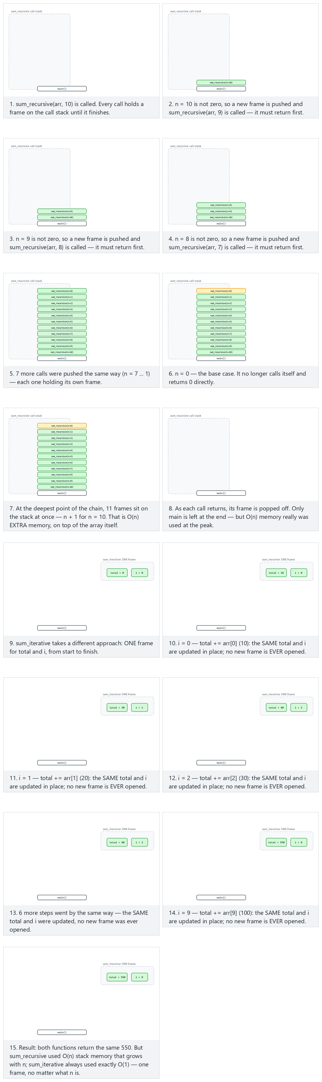
In the picker, also try 20 values with mixed signs (hard) and the edge cases 10 negative values and 22 values: deep recursion — or press 🎲 for random data at four difficulty levels, or type your own array.
int sum_recursive(const int arr[], int n) {
    if (n == 0)              /* base case: 0 elements left */
        return 0;
    return arr[n - 1] + sum_recursive(arr, n - 1);   /* one stack frame per call */
}

int sum_iterative(const int arr[], int n) {
    int total = 0;           /* ONE set of variables, reused every iteration */
    for (int i = 0; i < n; i++)
        total += arr[i];
    return total;
}
static int sumRecursive(int[] arr, int n) {
    if (n == 0)               // base case: 0 elements left
        return 0;
    return arr[n - 1] + sumRecursive(arr, n - 1);   // one stack frame per call
}

static int sumIterative(int[] arr, int n) {
    int total = 0;            // ONE set of variables, reused every iteration
    for (int i = 0; i < n; i++)
        total += arr[i];
    return total;
}
The full class (code/week-01/java/SpaceRecursiveVsIterative.java) mirrors the C program's four scenarios exactly.
Full program: space_recursive_vs_iterative.c / SpaceRecursiveVsIterative.java
/* Week 1 -- Introduction to Data Structures
 * Space complexity: a recursive sum pushes one stack frame per call;
 * an iterative sum reuses a single set of variables.
 * Runs the same normal / hard / edge-case scenarios as the space-recursive-vs-iterative animation.
 * CEN207 Data Structures (CS50-style lecture notes)
 */
#include <stdio.h>

int sum_recursive(const int arr[], int n) {
    if (n == 0)              /* base case: 0 elements left */
        return 0;
    return arr[n - 1] + sum_recursive(arr, n - 1);   /* one stack frame per call */
}

int sum_iterative(const int arr[], int n) {
    int total = 0;           /* ONE set of variables, reused every iteration */
    for (int i = 0; i < n; i++)
        total += arr[i];
    return total;
}

static void print_array(const int arr[], int n) {
    printf("arr:");
    for (int i = 0; i < n; i++)
        printf(" %d", arr[i]);
    printf("  (n = %d)\n", n);
}

static void run_scenario(const char *label, const int arr[], int n) {
    printf("-- %s --\n", label);
    print_array(arr, n);
    printf("sum_recursive -> %d (uses O(n) stack space: %d frames)\n", sum_recursive(arr, n), n);
    printf("sum_iterative -> %d (uses O(1) stack space: 1 frame, reused)\n\n", sum_iterative(arr, n));
}

int main(void) {
    /* normal: 10 positive values */
    int normal[] = {10, 20, 30, 40, 50, 60, 70, 80, 90, 100};
    run_scenario("normal: 10 positive values", normal, 10);

    /* hard: 20 values with mixed signs */
    int hard[] = {5, -3, 12, 8, -7, 15, 22, -10, 6, 18, 9, -4, 11, 27, -15, 3, 19, -8, 14, 7};
    run_scenario("hard: 20 values with mixed signs", hard, 20);

    /* edge: 10 negative values */
    int allNegative[] = {-5, -10, -15, -20, -25, -30, -35, -40, -45, -50};
    run_scenario("edge: 10 negative values", allNegative, 10);

    /* edge: 22 values, deep recursion */
    int deep[] = {1, 2, 3, 4, 5, 6, 7, 8, 9, 10, 11, 12, 13, 14, 15, 16, 17, 18, 19, 20, 21, 22};
    run_scenario("edge: 22 values, deep recursion", deep, 22);

    return 0;
}
/* Week 1 -- Introduction to Data Structures
 * Space complexity: a recursive sum pushes one stack frame per call;
 * an iterative sum reuses a single set of variables.
 * Runs the same normal / hard / edge-case scenarios as the space-recursive-vs-iterative animation.
 * CEN207 Data Structures (CS50-style lecture notes)
 */
public class SpaceRecursiveVsIterative {
    static int sumRecursive(int[] arr, int n) {
        if (n == 0)               // base case: 0 elements left
            return 0;
        return arr[n - 1] + sumRecursive(arr, n - 1);   // one stack frame per call
    }

    static int sumIterative(int[] arr, int n) {
        int total = 0;            // ONE set of variables, reused every iteration
        for (int i = 0; i < n; i++)
            total += arr[i];
        return total;
    }

    static void printArray(int[] arr) {
        StringBuilder sb = new StringBuilder("arr:");
        for (int v : arr) sb.append(' ').append(v);
        sb.append("  (n = ").append(arr.length).append(')');
        System.out.println(sb);
    }

    static void runScenario(String label, int[] arr) {
        System.out.println("-- " + label + " --");
        printArray(arr);
        int n = arr.length;
        System.out.println("sumRecursive -> " + sumRecursive(arr, n) + " (uses O(n) stack space: " + n + " frames)");
        System.out.println("sumIterative -> " + sumIterative(arr, n) + " (uses O(1) stack space: 1 frame, reused)");
        System.out.println();
    }

    public static void main(String[] args) {
        // normal: 10 positive values
        int[] normal = {10, 20, 30, 40, 50, 60, 70, 80, 90, 100};
        runScenario("normal: 10 positive values", normal);

        // hard: 20 values with mixed signs
        int[] hard = {5, -3, 12, 8, -7, 15, 22, -10, 6, 18, 9, -4, 11, 27, -15, 3, 19, -8, 14, 7};
        runScenario("hard: 20 values with mixed signs", hard);

        // edge: 10 negative values
        int[] allNegative = {-5, -10, -15, -20, -25, -30, -35, -40, -45, -50};
        runScenario("edge: 10 negative values", allNegative);

        // edge: 22 values, deep recursion
        int[] deep = {1, 2, 3, 4, 5, 6, 7, 8, 9, 10, 11, 12, 13, 14, 15, 16, 17, 18, 19, 20, 21, 22};
        runScenario("edge: 22 values, deep recursion", deep);
    }
}
Full program: space_recursive_vs_iterative.c / SpaceRecursiveVsIterative.java
/* Week 1 -- Introduction to Data Structures
 * Space complexity: a recursive sum pushes one stack frame per call;
 * an iterative sum reuses a single set of variables.
 * Runs the same normal / hard / edge-case scenarios as the space-recursive-vs-iterative animation.
 * CEN207 Data Structures (CS50-style lecture notes)
 */
#include <stdio.h>

int sum_recursive(const int arr[], int n) {
    if (n == 0)              /* base case: 0 elements left */
        return 0;
    return arr[n - 1] + sum_recursive(arr, n - 1);   /* one stack frame per call */
}

int sum_iterative(const int arr[], int n) {
    int total = 0;           /* ONE set of variables, reused every iteration */
    for (int i = 0; i < n; i++)
        total += arr[i];
    return total;
}

static void print_array(const int arr[], int n) {
    printf("arr:");
    for (int i = 0; i < n; i++)
        printf(" %d", arr[i]);
    printf("  (n = %d)\n", n);
}

static void run_scenario(const char *label, const int arr[], int n) {
    printf("-- %s --\n", label);
    print_array(arr, n);
    printf("sum_recursive -> %d (uses O(n) stack space: %d frames)\n", sum_recursive(arr, n), n);
    printf("sum_iterative -> %d (uses O(1) stack space: 1 frame, reused)\n\n", sum_iterative(arr, n));
}

int main(void) {
    /* normal: 10 positive values */
    int normal[] = {10, 20, 30, 40, 50, 60, 70, 80, 90, 100};
    run_scenario("normal: 10 positive values", normal, 10);

    /* hard: 20 values with mixed signs */
    int hard[] = {5, -3, 12, 8, -7, 15, 22, -10, 6, 18, 9, -4, 11, 27, -15, 3, 19, -8, 14, 7};
    run_scenario("hard: 20 values with mixed signs", hard, 20);

    /* edge: 10 negative values */
    int allNegative[] = {-5, -10, -15, -20, -25, -30, -35, -40, -45, -50};
    run_scenario("edge: 10 negative values", allNegative, 10);

    /* edge: 22 values, deep recursion */
    int deep[] = {1, 2, 3, 4, 5, 6, 7, 8, 9, 10, 11, 12, 13, 14, 15, 16, 17, 18, 19, 20, 21, 22};
    run_scenario("edge: 22 values, deep recursion", deep, 22);

    return 0;
}
/* Week 1 -- Introduction to Data Structures
 * Space complexity: a recursive sum pushes one stack frame per call;
 * an iterative sum reuses a single set of variables.
 * Runs the same normal / hard / edge-case scenarios as the space-recursive-vs-iterative animation.
 * CEN207 Data Structures (CS50-style lecture notes)
 */
public class SpaceRecursiveVsIterative {
    static int sumRecursive(int[] arr, int n) {
        if (n == 0)               // base case: 0 elements left
            return 0;
        return arr[n - 1] + sumRecursive(arr, n - 1);   // one stack frame per call
    }

    static int sumIterative(int[] arr, int n) {
        int total = 0;            // ONE set of variables, reused every iteration
        for (int i = 0; i < n; i++)
            total += arr[i];
        return total;
    }

    static void printArray(int[] arr) {
        StringBuilder sb = new StringBuilder("arr:");
        for (int v : arr) sb.append(' ').append(v);
        sb.append("  (n = ").append(arr.length).append(')');
        System.out.println(sb);
    }

    static void runScenario(String label, int[] arr) {
        System.out.println("-- " + label + " --");
        printArray(arr);
        int n = arr.length;
        System.out.println("sumRecursive -> " + sumRecursive(arr, n) + " (uses O(n) stack space: " + n + " frames)");
        System.out.println("sumIterative -> " + sumIterative(arr, n) + " (uses O(1) stack space: 1 frame, reused)");
        System.out.println();
    }

    public static void main(String[] args) {
        // normal: 10 positive values
        int[] normal = {10, 20, 30, 40, 50, 60, 70, 80, 90, 100};
        runScenario("normal: 10 positive values", normal);

        // hard: 20 values with mixed signs
        int[] hard = {5, -3, 12, 8, -7, 15, 22, -10, 6, 18, 9, -4, 11, 27, -15, 3, 19, -8, 14, 7};
        runScenario("hard: 20 values with mixed signs", hard);

        // edge: 10 negative values
        int[] allNegative = {-5, -10, -15, -20, -25, -30, -35, -40, -45, -50};
        runScenario("edge: 10 negative values", allNegative);

        // edge: 22 values, deep recursion
        int[] deep = {1, 2, 3, 4, 5, 6, 7, 8, 9, 10, 11, 12, 13, 14, 15, 16, 17, 18, 19, 20, 21, 22};
        runScenario("edge: 22 values, deep recursion", deep);
    }
}
Try it
Expected output:
-- normal: 10 positive values --
arr: 10 20 30 40 50 60 70 80 90 100  (n = 10)
sum_recursive -> 550 (uses O(n) stack space: 10 frames)
sum_iterative -> 550 (uses O(1) stack space: 1 frame, reused)

-- hard: 20 values with mixed signs --
arr: 5 -3 12 8 -7 15 22 -10 6 18 9 -4 11 27 -15 3 19 -8 14 7  (n = 20)
sum_recursive -> 129 (uses O(n) stack space: 20 frames)
sum_iterative -> 129 (uses O(1) stack space: 1 frame, reused)

-- edge: 10 negative values --
arr: -5 -10 -15 -20 -25 -30 -35 -40 -45 -50  (n = 10)
sum_recursive -> -275 (uses O(n) stack space: 10 frames)
sum_iterative -> -275 (uses O(1) stack space: 1 frame, reused)

-- edge: 22 values, deep recursion --
arr: 1 2 3 4 5 6 7 8 9 10 11 12 13 14 15 16 17 18 19 20 21 22  (n = 22)
sum_recursive -> 253 (uses O(n) stack space: 22 frames)
sum_iterative -> 253 (uses O(1) stack space: 1 frame, reused)
Expected output (identical values, sumRecursive/sumIterative naming):
-- normal: 10 positive values --
arr: 10 20 30 40 50 60 70 80 90 100  (n = 10)
sumRecursive -> 550 (uses O(n) stack space: 10 frames)
sumIterative -> 550 (uses O(1) stack space: 1 frame, reused)

-- hard: 20 values with mixed signs --
arr: 5 -3 12 8 -7 15 22 -10 6 18 9 -4 11 27 -15 3 19 -8 14 7  (n = 20)
sumRecursive -> 129 (uses O(n) stack space: 20 frames)
sumIterative -> 129 (uses O(1) stack space: 1 frame, reused)

-- edge: 10 negative values --
arr: -5 -10 -15 -20 -25 -30 -35 -40 -45 -50  (n = 10)
sumRecursive -> -275 (uses O(n) stack space: 10 frames)
sumIterative -> -275 (uses O(1) stack space: 1 frame, reused)

-- edge: 22 values, deep recursion --
arr: 1 2 3 4 5 6 7 8 9 10 11 12 13 14 15 16 17 18 19 20 21 22  (n = 22)
sumRecursive -> 253 (uses O(n) stack space: 22 frames)
sumIterative -> 253 (uses O(1) stack space: 1 frame, reused)
Every scenario returns the same value from both functions. sum_recursive peaks at n simultaneous stack frames (22 for the deep scenario) — grow the array and the peak grows with it, one frame per element: O(n). sum_iterative never has more than the one frame main calls it with, no matter how large n gets: O(1).
Common mistakes
- Reading Big-O off the code instead of the steps. A single line can hide a loop (
arr.contains(x)inside a loop is O(n) inside another O(n) loop = O(n²) overall) — always ask what the line actually does, not how many characters it takes to write. - Forgetting that Big-O needs a sorted input for binary search. Running binary search on unsorted data gives wrong answers, not just slow ones — the halving logic assumes order.
- Confusing "O(1)" with "instant" or "free". O(1) means the cost does not grow with
n; it can still be a slow constant (reading a value from a network call is O(1) innand still slower than an in-memory O(log n) search for any n you will meet in this course). - Quoting only the worst case and ignoring that average case can matter more in practice (and vice versa) — state which case you mean.
Test yourself: performance analysis
1. An algorithm does exactly 5n + 20 basic operations. What is its Big-O?
O(n). Drop the constant factor (5) and the additive constant (20); only the fastest-growing term, n, survives.
2. Why can binary search not be used directly on a linked list the way it is used on an array?
Binary search needs O(1) access to the middle element by index. An array gives that directly (arr[mid]); a linked list (Week 2) must be walked node by node to reach position mid, which is already O(n) — that single step would erase binary search's entire advantage.
3. Which case — best, worst, or average — does "Big-O of an algorithm" usually refer to when stated without qualification?
The worst case: the guaranteed upper bound, useful precisely because it holds no matter what input you are given.
4. Pointers and objects for data and variables
4.1 A question to start
Write a function swap(a, b) that exchanges the values of two variables in the caller. In many languages this is surprisingly impossible to write directly — the function only ever sees copies of a and b, and swapping the copies does nothing to the originals. To actually reach back into the caller's variables, the function needs the location of each variable, not just its value. That location is a pointer.
4.2 A short history
The idea of a variable that holds another variable's address goes back to assembly language and to early systems languages: BCPL (Martin Richards, 1966) and B (Ken Thompson, 1969) already had address-of and dereference operations, and Dennis Ritchie's C (1972) — BCPL and B's direct descendant — made the pointer, and struct pointers in particular, central to how the language is used. Java (James Gosling and others, first released 1995) deliberately removed raw pointers and pointer arithmetic from the language, replacing them with references: you can still have two variables name the same object, but you can no longer compute an arbitrary address or step a pointer past the end of an array. Section 4.6 and the animations below show exactly what that trade gains and costs.
4.3 Intuition: memory as numbered mailboxes
Picture memory as a long street of numbered mailboxes. A variable is a mailbox: it has an address (its number) and contents (the value inside). int x = 3; puts 3 in some mailbox — say, number 1000. &x asks "what is x's mailbox number?" and gets 1000. A pointer is a mailbox whose contents are themselves a mailbox number — a pointer variable p can hold 1000, meaning "go look at mailbox 1000". Reading through a pointer (dereferencing, written *p) means: go to the mailbox number stored in p, and read (or write) what is there.
4.4 The pointer operations
| Operation | Syntax | What it does | Complexity |
|---|---|---|---|
| Address-of | &x | Produces the address of variable x | O(1) |
| Declare a pointer | int *p; | Declares p as a variable that will hold an address of an int | O(1) |
| Assign an address | p = &x; | Stores x's address in p; p now "points to" x | O(1) |
| Dereference (read) | *p | Follows p to its target and reads the value there | O(1) |
| Dereference (write) | *p = v; | Follows p to its target and writes v there | O(1) |
| Pointer arithmetic | p + k | Computes a new address k * sizeof(*p) bytes ahead of p, without changing p (Section 4.7) | O(1) |
Every one of these is O(1): following a pointer, or computing a new address from one, is always a single jump or a single multiply-and-add, never a search — this is exactly why pointers (and, in Week 2, the linked structures built from them) are efficient.
4.5 A variable, its address, and a pointer
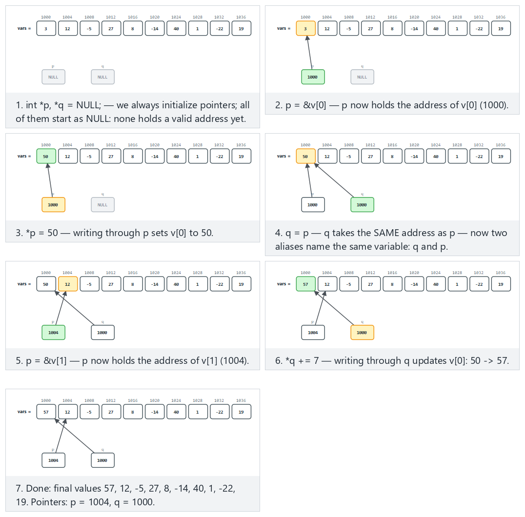
/* Week 1 -- Introduction to Data Structures
 * A variable, its address, and a pointer that stores that address.
 * CEN207 Data Structures (CS50-style lecture notes)
 */
#include <stdio.h>

int main(void) {
    int x = 3;
    int *p = &x;

    printf("x = %d, stored at address %p\n", x, (void *) &x);
    printf("p = %p (p holds the address of x)\n", (void *) p);
    printf("*p = %d (dereferencing p reads the value at that address)\n", *p);

    *p = 5;
    printf("after *p = 5: x = %d\n", x);

    return 0;
}
/* Week 1 -- Introduction to Data Structures
 * Java has no raw pointers, but arrays and objects are REFERENCE types:
 * a variable holds a reference to the data, not the data itself.
 * CEN207 Data Structures (CS50-style lecture notes)
 */
public class ReferenceBasics {
    public static void main(String[] args) {
        int x = 3;                 // a plain int: the VALUE 3 is stored directly
        int[] box = {3};           // an array: box is a REFERENCE to a one-element block

        System.out.println("x = " + x);
        System.out.println("box[0] = " + box[0] + " (box holds a reference to the array)");

        int[] alias = box;         // alias refers to the SAME array as box, not a copy
        alias[0] = 5;               // writing through alias is visible through box too
        System.out.println("after alias[0] = 5: box[0] = " + box[0]);

        int y = x;                  // y is an independent COPY of x's value
        y = 99;
        System.out.println("after y = 99: x = " + x + " (unchanged, x and y are independent)");
    }
}
Try it
Expected output (your addresses will be different — the pattern is what matters, not the exact numbers):
Notice the two halves of the Java program tell opposite stories with the same syntax int[] alias = box; versus int y = x;: box is an array, a reference type, so alias becomes a second name for the same array — exactly like p pointing at x in C. But x is a primitive int, a value type, so y = x; copies the value — changing y never touches x. C's pointers make this distinction explicit and controllable (int x vs int *p); Java makes the same distinction implicit in the type (int vs int[]/object types) and never lets you turn one into the other.
4.6 Pointer to a struct, and ->
A struct groups related fields into one value; a pointer to a struct lets you reach — and modify — the original struct through that pointer, not a copy of it. Writing (*p).field (dereference first, then access a field) is so common that C gives it a shorthand: p->field.
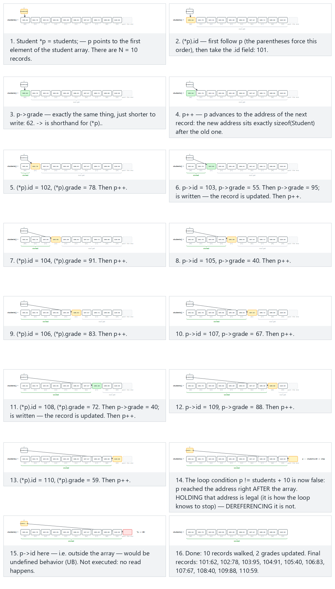
/* Week 1 -- Introduction to Data Structures
 * A pointer to a struct, and the -> shorthand for (*p).field.
 * CEN207 Data Structures (CS50-style lecture notes)
 */
#include <stdio.h>

typedef struct Point {
    int x;
    int y;
} Point;

int main(void) {
    Point a = {3, 4};
    Point *p = &a;

    printf("a = (%d, %d)\n", a.x, a.y);
    printf("(*p).x = %d, p->x = %d (same value, -> is shorthand)\n", (*p).x, p->x);

    p->x = 10;
    printf("after p->x = 10: a = (%d, %d)\n", a.x, a.y);

    return 0;
}
/* Week 1 -- Introduction to Data Structures
 * A reference to an object, and the '.' access that plays the role of C's '->'.
 * CEN207 Data Structures (CS50-style lecture notes)
 */
public class PointRef {
    static class Point {
        int x;
        int y;
        Point(int x, int y) { this.x = x; this.y = y; }
    }

    public static void main(String[] args) {
        Point a = new Point(3, 4);
        Point p = a;                // p is another reference to the SAME object as a

        System.out.println("a = (" + a.x + ", " + a.y + ")");
        System.out.println("p.x = " + p.x + " (same object as a, reached through p)");

        p.x = 10;
        System.out.println("after p.x = 10: a = (" + a.x + ", " + a.y + ")");
    }
}
Try it
Expected output:
Java has no -> at all, and does not need one: every object variable is already a reference, so . always means "follow the reference, then access the field" — there is no separate "dereference first" step to write out.
4.7 Pointer arithmetic: p + k means k * sizeof(*p)
Section 4.4 listed *p — dereferencing a pointer — as O(1). There is a second pointer operation that looks like plain arithmetic but is not: p + k. It does not move k bytes forward; it moves k * sizeof(*p) bytes forward, because the compiler knows the type p points to and scales the offset for you. p + k also never changes p itself — it computes a new address, which *(p + k) then dereferences.
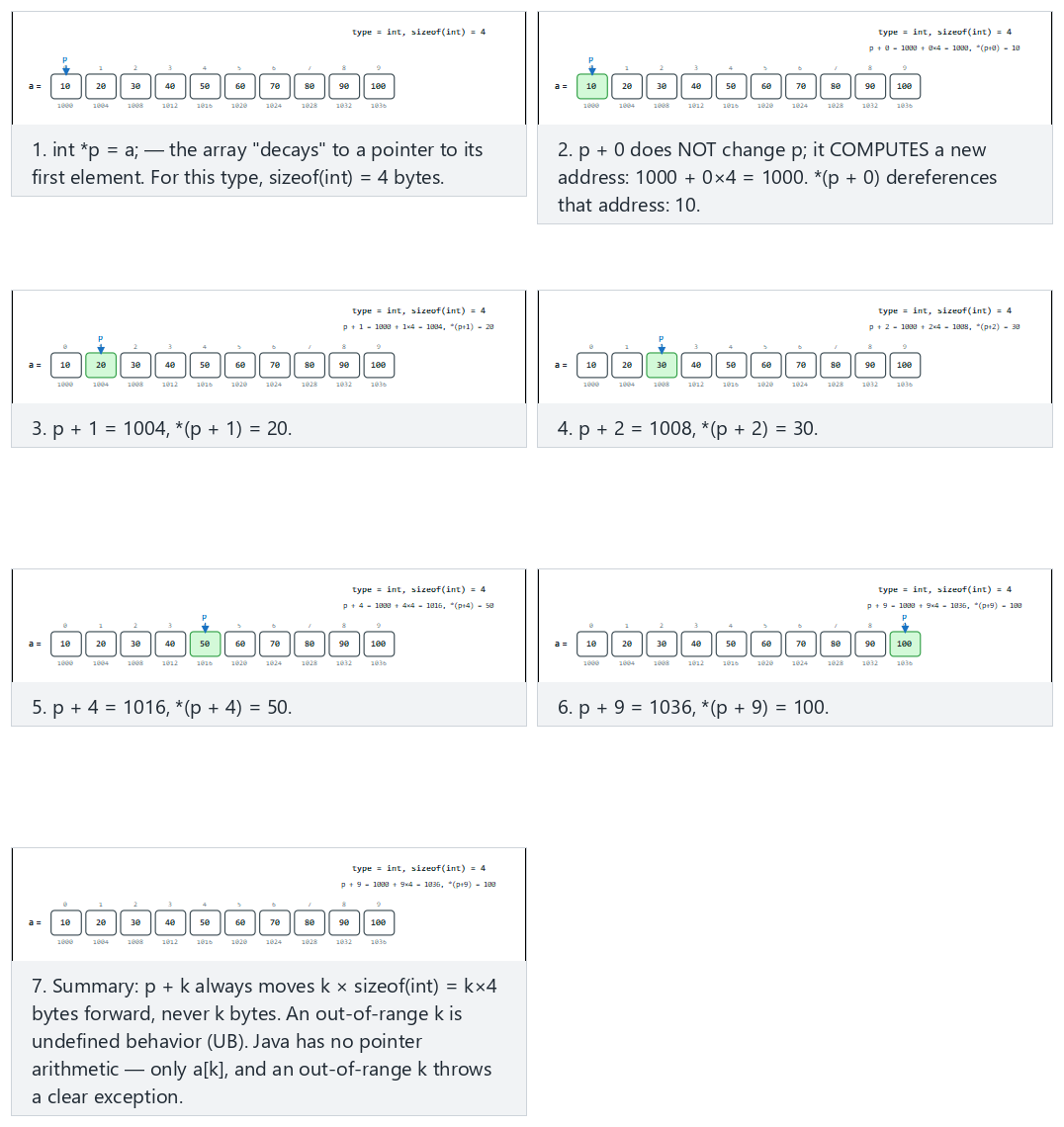
In the picker, also try double array (sizeof = 8), 7 offsets (hard) and the edge cases out-of-range offsets: negative and beyond N and char array (sizeof = 1): p + k coincides with k bytes — or press 🎲 for random data (and a random type) at four difficulty levels, or type your own array, type and offsets.
int *p = a;                  /* array decays to a pointer to its first element */

if (k < 0 || k >= N) {
    /* p + k lands outside a[]: reading *(p + k) is undefined behavior (UB) */
} else {
    void *addr = (void *) (p + k);   /* address + k * sizeof(int) */
    int v = *(p + k);                /* dereference: read the value at that address */
}
// Java has no pointer arithmetic; indices are the only way to move between elements
if (k < 0 || k >= N) {
    // out of range: throws ArrayIndexOutOfBoundsException, not undefined behaviour
} else {
    int v = a[k];             // a[k] is the closest Java equivalent of *(p + k)
}
The full class (code/week-01/java/ArrayIndexing.java) mirrors the C program's four scenarios, printing the same base + k * sizeof(type) arithmetic for comparison even though Java itself only ever indexes with a[k].
Full program: pointer_arithmetic.c / ArrayIndexing.java
/* Week 1 -- Introduction to Data Structures
 * Pointer arithmetic: p + k means base address + k * sizeof(*p), never k bytes.
 * An out-of-range k is undefined behavior (UB); the guard below reports it instead of reading it.
 * Addresses are a PRETEND base (matching the animation), not real OS addresses, so the output is
 * reproducible and can be compared byte for byte with the Java version.
 * Runs the same normal / hard / edge-case scenarios as the pointer-arithmetic animation.
 * CEN207 Data Structures (CS50-style lecture notes)
 */
#include <stdio.h>

static void run_int_scenario(const char *label, long base, const int values[], int n,
                              const int offsets[], int offCount) {
    printf("-- %s (type = int, sizeof = %zu) --\n", label, sizeof(int));
    const int *p = values;   /* p decays to point at values[0] */
    for (int i = 0; i < offCount; i++) {
        int k = offsets[i];
        if (k < 0 || k >= n) {
            printf("p + %d -> out of range (UB): 0 <= k < %d required\n", k, n);
            continue;
        }
        long addr = base + (long) k * (long) sizeof(int);
        printf("p + %d = %ld, *(p + %d) = %d\n", k, addr, k, *(p + k));
    }
    printf("\n");
}

static void run_double_scenario(const char *label, long base, const double values[], int n,
                                 const int offsets[], int offCount) {
    printf("-- %s (type = double, sizeof = %zu) --\n", label, sizeof(double));
    const double *p = values;
    for (int i = 0; i < offCount; i++) {
        int k = offsets[i];
        if (k < 0 || k >= n) {
            printf("p + %d -> out of range (UB): 0 <= k < %d required\n", k, n);
            continue;
        }
        long addr = base + (long) k * (long) sizeof(double);
        printf("p + %d = %ld, *(p + %d) = %.0f\n", k, addr, k, *(p + k));
    }
    printf("\n");
}

static void run_char_scenario(const char *label, long base, const char values[], int n,
                               const int offsets[], int offCount) {
    printf("-- %s (type = char, sizeof = %zu) --\n", label, sizeof(char));
    const char *p = values;
    for (int i = 0; i < offCount; i++) {
        int k = offsets[i];
        if (k < 0 || k >= n) {
            printf("p + %d -> out of range (UB): 0 <= k < %d required\n", k, n);
            continue;
        }
        long addr = base + (long) k * (long) sizeof(char);   /* sizeof(char) is always 1 */
        printf("p + %d = %ld, *(p + %d) = %d\n", k, addr, k, (int) *(p + k));
    }
    printf("\n");
}

int main(void) {
    /* normal: int array, 5 valid offsets */
    int normalValues[] = {10, 20, 30, 40, 50, 60, 70, 80, 90, 100};
    int normalOffsets[] = {0, 1, 2, 4, 9};
    run_int_scenario("normal: int array, 5 valid offsets", 1000, normalValues, 10, normalOffsets, 5);

    /* hard: double array (sizeof = 8), 7 offsets */
    double hardValues[] = {1, 2, 3, 4, 5, 6, 7, 8, 9, 10, 11, 12};
    int hardOffsets[] = {0, 2, 5, 8, 11, 6, 3};
    run_double_scenario("hard: double array (sizeof = 8), 7 offsets", 2000, hardValues, 12, hardOffsets, 7);

    /* edge: out-of-range offsets, negative and beyond N */
    int edgeValues[] = {4, 8, 15, 16, 23, 42, 8, 9, 15, 3};
    int edgeOffsets[] = {-1, 0, 5, 10, 15};
    run_int_scenario("edge: out-of-range offsets (negative and beyond N)", 1000, edgeValues, 10, edgeOffsets, 5);

    /* edge: char array (sizeof = 1), p + k coincides with k bytes */
    char charValues[] = {65, 66, 67, 68, 69, 70, 71, 72, 73, 74};
    int charOffsets[] = {0, 1, 2, 3, 4, 5, 6, 7, 8, 9};
    run_char_scenario("edge: char array (sizeof = 1)", 500, charValues, 10, charOffsets, 10);

    return 0;
}
/* Week 1 -- Introduction to Data Structures
 * Java has no pointer arithmetic -- array indexing is the only way to move between elements.
 * These scenarios still print the SAME "address = base + k * sizeof(type)" arithmetic as the C
 * version, using the type's C size, purely to compare the formula's result side by side; Java
 * itself never computes a real address, it only ever indexes with a[k].
 * Runs the same normal / hard / edge-case scenarios as the pointer-arithmetic animation.
 * CEN207 Data Structures (CS50-style lecture notes)
 */
public class ArrayIndexing {
    static void runIntScenario(String label, long base, int[] values, int[] offsets) {
        int n = values.length, sizeofInt = 4;
        System.out.println("-- " + label + " (type = int, sizeof = " + sizeofInt + ") --");
        for (int k : offsets) {
            if (k < 0 || k >= n) {
                System.out.println("a[" + k + "] -> out of range: throws ArrayIndexOutOfBoundsException in real Java");
                continue;
            }
            long addr = base + (long) k * sizeofInt;
            System.out.println("p + " + k + " = " + addr + ", a[" + k + "] = " + values[k]);
        }
        System.out.println();
    }

    static void runDoubleScenario(String label, long base, double[] values, int[] offsets) {
        int n = values.length, sizeofDouble = 8;
        System.out.println("-- " + label + " (type = double, sizeof = " + sizeofDouble + ") --");
        for (int k : offsets) {
            if (k < 0 || k >= n) {
                System.out.println("a[" + k + "] -> out of range: throws ArrayIndexOutOfBoundsException in real Java");
                continue;
            }
            long addr = base + (long) k * sizeofDouble;
            System.out.printf("p + %d = %d, a[%d] = %.0f%n", k, addr, k, values[k]);
        }
        System.out.println();
    }

    static void runCharScenario(String label, long base, char[] values, int[] offsets) {
        int n = values.length, sizeofChar = 1;
        System.out.println("-- " + label + " (type = char, sizeof = " + sizeofChar + ") --");
        for (int k : offsets) {
            if (k < 0 || k >= n) {
                System.out.println("a[" + k + "] -> out of range: throws ArrayIndexOutOfBoundsException in real Java");
                continue;
            }
            long addr = base + (long) k * sizeofChar;
            System.out.println("p + " + k + " = " + addr + ", a[" + k + "] = " + (int) values[k]);
        }
        System.out.println();
    }

    public static void main(String[] args) {
        // normal: int array, 5 valid offsets
        int[] normalValues = {10, 20, 30, 40, 50, 60, 70, 80, 90, 100};
        int[] normalOffsets = {0, 1, 2, 4, 9};
        runIntScenario("normal: int array, 5 valid offsets", 1000, normalValues, normalOffsets);

        // hard: double array (sizeof = 8), 7 offsets
        double[] hardValues = {1, 2, 3, 4, 5, 6, 7, 8, 9, 10, 11, 12};
        int[] hardOffsets = {0, 2, 5, 8, 11, 6, 3};
        runDoubleScenario("hard: double array (sizeof = 8), 7 offsets", 2000, hardValues, hardOffsets);

        // edge: out-of-range offsets, negative and beyond N
        int[] edgeValues = {4, 8, 15, 16, 23, 42, 8, 9, 15, 3};
        int[] edgeOffsets = {-1, 0, 5, 10, 15};
        runIntScenario("edge: out-of-range offsets (negative and beyond N)", 1000, edgeValues, edgeOffsets);

        // edge: char array (sizeof = 1), p + k coincides with k bytes
        char[] charValues = {65, 66, 67, 68, 69, 70, 71, 72, 73, 74};
        int[] charOffsets = {0, 1, 2, 3, 4, 5, 6, 7, 8, 9};
        runCharScenario("edge: char array (sizeof = 1)", 500, charValues, charOffsets);
    }
}
Full program: pointer_arithmetic.c / ArrayIndexing.java
/* Week 1 -- Introduction to Data Structures
 * Pointer arithmetic: p + k means base address + k * sizeof(*p), never k bytes.
 * An out-of-range k is undefined behavior (UB); the guard below reports it instead of reading it.
 * Addresses are a PRETEND base (matching the animation), not real OS addresses, so the output is
 * reproducible and can be compared byte for byte with the Java version.
 * Runs the same normal / hard / edge-case scenarios as the pointer-arithmetic animation.
 * CEN207 Data Structures (CS50-style lecture notes)
 */
#include <stdio.h>

static void run_int_scenario(const char *label, long base, const int values[], int n,
                              const int offsets[], int offCount) {
    printf("-- %s (type = int, sizeof = %zu) --\n", label, sizeof(int));
    const int *p = values;   /* p decays to point at values[0] */
    for (int i = 0; i < offCount; i++) {
        int k = offsets[i];
        if (k < 0 || k >= n) {
            printf("p + %d -> out of range (UB): 0 <= k < %d required\n", k, n);
            continue;
        }
        long addr = base + (long) k * (long) sizeof(int);
        printf("p + %d = %ld, *(p + %d) = %d\n", k, addr, k, *(p + k));
    }
    printf("\n");
}

static void run_double_scenario(const char *label, long base, const double values[], int n,
                                 const int offsets[], int offCount) {
    printf("-- %s (type = double, sizeof = %zu) --\n", label, sizeof(double));
    const double *p = values;
    for (int i = 0; i < offCount; i++) {
        int k = offsets[i];
        if (k < 0 || k >= n) {
            printf("p + %d -> out of range (UB): 0 <= k < %d required\n", k, n);
            continue;
        }
        long addr = base + (long) k * (long) sizeof(double);
        printf("p + %d = %ld, *(p + %d) = %.0f\n", k, addr, k, *(p + k));
    }
    printf("\n");
}

static void run_char_scenario(const char *label, long base, const char values[], int n,
                               const int offsets[], int offCount) {
    printf("-- %s (type = char, sizeof = %zu) --\n", label, sizeof(char));
    const char *p = values;
    for (int i = 0; i < offCount; i++) {
        int k = offsets[i];
        if (k < 0 || k >= n) {
            printf("p + %d -> out of range (UB): 0 <= k < %d required\n", k, n);
            continue;
        }
        long addr = base + (long) k * (long) sizeof(char);   /* sizeof(char) is always 1 */
        printf("p + %d = %ld, *(p + %d) = %d\n", k, addr, k, (int) *(p + k));
    }
    printf("\n");
}

int main(void) {
    /* normal: int array, 5 valid offsets */
    int normalValues[] = {10, 20, 30, 40, 50, 60, 70, 80, 90, 100};
    int normalOffsets[] = {0, 1, 2, 4, 9};
    run_int_scenario("normal: int array, 5 valid offsets", 1000, normalValues, 10, normalOffsets, 5);

    /* hard: double array (sizeof = 8), 7 offsets */
    double hardValues[] = {1, 2, 3, 4, 5, 6, 7, 8, 9, 10, 11, 12};
    int hardOffsets[] = {0, 2, 5, 8, 11, 6, 3};
    run_double_scenario("hard: double array (sizeof = 8), 7 offsets", 2000, hardValues, 12, hardOffsets, 7);

    /* edge: out-of-range offsets, negative and beyond N */
    int edgeValues[] = {4, 8, 15, 16, 23, 42, 8, 9, 15, 3};
    int edgeOffsets[] = {-1, 0, 5, 10, 15};
    run_int_scenario("edge: out-of-range offsets (negative and beyond N)", 1000, edgeValues, 10, edgeOffsets, 5);

    /* edge: char array (sizeof = 1), p + k coincides with k bytes */
    char charValues[] = {65, 66, 67, 68, 69, 70, 71, 72, 73, 74};
    int charOffsets[] = {0, 1, 2, 3, 4, 5, 6, 7, 8, 9};
    run_char_scenario("edge: char array (sizeof = 1)", 500, charValues, 10, charOffsets, 10);

    return 0;
}
/* Week 1 -- Introduction to Data Structures
 * Java has no pointer arithmetic -- array indexing is the only way to move between elements.
 * These scenarios still print the SAME "address = base + k * sizeof(type)" arithmetic as the C
 * version, using the type's C size, purely to compare the formula's result side by side; Java
 * itself never computes a real address, it only ever indexes with a[k].
 * Runs the same normal / hard / edge-case scenarios as the pointer-arithmetic animation.
 * CEN207 Data Structures (CS50-style lecture notes)
 */
public class ArrayIndexing {
    static void runIntScenario(String label, long base, int[] values, int[] offsets) {
        int n = values.length, sizeofInt = 4;
        System.out.println("-- " + label + " (type = int, sizeof = " + sizeofInt + ") --");
        for (int k : offsets) {
            if (k < 0 || k >= n) {
                System.out.println("a[" + k + "] -> out of range: throws ArrayIndexOutOfBoundsException in real Java");
                continue;
            }
            long addr = base + (long) k * sizeofInt;
            System.out.println("p + " + k + " = " + addr + ", a[" + k + "] = " + values[k]);
        }
        System.out.println();
    }

    static void runDoubleScenario(String label, long base, double[] values, int[] offsets) {
        int n = values.length, sizeofDouble = 8;
        System.out.println("-- " + label + " (type = double, sizeof = " + sizeofDouble + ") --");
        for (int k : offsets) {
            if (k < 0 || k >= n) {
                System.out.println("a[" + k + "] -> out of range: throws ArrayIndexOutOfBoundsException in real Java");
                continue;
            }
            long addr = base + (long) k * sizeofDouble;
            System.out.printf("p + %d = %d, a[%d] = %.0f%n", k, addr, k, values[k]);
        }
        System.out.println();
    }

    static void runCharScenario(String label, long base, char[] values, int[] offsets) {
        int n = values.length, sizeofChar = 1;
        System.out.println("-- " + label + " (type = char, sizeof = " + sizeofChar + ") --");
        for (int k : offsets) {
            if (k < 0 || k >= n) {
                System.out.println("a[" + k + "] -> out of range: throws ArrayIndexOutOfBoundsException in real Java");
                continue;
            }
            long addr = base + (long) k * sizeofChar;
            System.out.println("p + " + k + " = " + addr + ", a[" + k + "] = " + (int) values[k]);
        }
        System.out.println();
    }

    public static void main(String[] args) {
        // normal: int array, 5 valid offsets
        int[] normalValues = {10, 20, 30, 40, 50, 60, 70, 80, 90, 100};
        int[] normalOffsets = {0, 1, 2, 4, 9};
        runIntScenario("normal: int array, 5 valid offsets", 1000, normalValues, normalOffsets);

        // hard: double array (sizeof = 8), 7 offsets
        double[] hardValues = {1, 2, 3, 4, 5, 6, 7, 8, 9, 10, 11, 12};
        int[] hardOffsets = {0, 2, 5, 8, 11, 6, 3};
        runDoubleScenario("hard: double array (sizeof = 8), 7 offsets", 2000, hardValues, hardOffsets);

        // edge: out-of-range offsets, negative and beyond N
        int[] edgeValues = {4, 8, 15, 16, 23, 42, 8, 9, 15, 3};
        int[] edgeOffsets = {-1, 0, 5, 10, 15};
        runIntScenario("edge: out-of-range offsets (negative and beyond N)", 1000, edgeValues, edgeOffsets);

        // edge: char array (sizeof = 1), p + k coincides with k bytes
        char[] charValues = {65, 66, 67, 68, 69, 70, 71, 72, 73, 74};
        int[] charOffsets = {0, 1, 2, 3, 4, 5, 6, 7, 8, 9};
        runCharScenario("edge: char array (sizeof = 1)", 500, charValues, charOffsets);
    }
}
Try it
Expected output:
-- normal: int array, 5 valid offsets (type = int, sizeof = 4) --
p + 0 = 1000, *(p + 0) = 10
p + 1 = 1004, *(p + 1) = 20
p + 2 = 1008, *(p + 2) = 30
p + 4 = 1016, *(p + 4) = 50
p + 9 = 1036, *(p + 9) = 100

-- hard: double array (sizeof = 8), 7 offsets (type = double, sizeof = 8) --
p + 0 = 2000, *(p + 0) = 1
p + 2 = 2016, *(p + 2) = 3
p + 5 = 2040, *(p + 5) = 6
p + 8 = 2064, *(p + 8) = 9
p + 11 = 2088, *(p + 11) = 12
p + 6 = 2048, *(p + 6) = 7
p + 3 = 2024, *(p + 3) = 4

-- edge: out-of-range offsets (negative and beyond N) (type = int, sizeof = 4) --
p + -1 -> out of range (UB): 0 <= k < 10 required
p + 0 = 1000, *(p + 0) = 4
p + 5 = 1020, *(p + 5) = 42
p + 10 -> out of range (UB): 0 <= k < 10 required
p + 15 -> out of range (UB): 0 <= k < 10 required

-- edge: char array (sizeof = 1) (type = char, sizeof = 1) --
p + 0 = 500, *(p + 0) = 65
p + 1 = 501, *(p + 1) = 66
p + 2 = 502, *(p + 2) = 67
p + 3 = 503, *(p + 3) = 68
p + 4 = 504, *(p + 4) = 69
p + 5 = 505, *(p + 5) = 70
p + 6 = 506, *(p + 6) = 71
p + 7 = 507, *(p + 7) = 72
p + 8 = 508, *(p + 8) = 73
p + 9 = 509, *(p + 9) = 74
Expected output (same values and addresses; a[k] where C prints *(p + k), and a plain message instead of UB for out-of-range offsets, since Java throws instead of doing whatever the hardware does):
-- normal: int array, 5 valid offsets (type = int, sizeof = 4) --
p + 0 = 1000, a[0] = 10
p + 1 = 1004, a[1] = 20
p + 2 = 1008, a[2] = 30
p + 4 = 1016, a[4] = 50
p + 9 = 1036, a[9] = 100

-- hard: double array (sizeof = 8), 7 offsets (type = double, sizeof = 8) --
p + 0 = 2000, a[0] = 1
p + 2 = 2016, a[2] = 3
p + 5 = 2040, a[5] = 6
p + 8 = 2064, a[8] = 9
p + 11 = 2088, a[11] = 12
p + 6 = 2048, a[6] = 7
p + 3 = 2024, a[3] = 4

-- edge: out-of-range offsets (negative and beyond N) (type = int, sizeof = 4) --
a[-1] -> out of range: throws ArrayIndexOutOfBoundsException in real Java
p + 0 = 1000, a[0] = 4
p + 5 = 1020, a[5] = 42
a[10] -> out of range: throws ArrayIndexOutOfBoundsException in real Java
a[15] -> out of range: throws ArrayIndexOutOfBoundsException in real Java

-- edge: char array (sizeof = 1) (type = char, sizeof = 1) --
p + 0 = 500, a[0] = 65
p + 1 = 501, a[1] = 66
p + 2 = 502, a[2] = 67
p + 3 = 503, a[3] = 68
p + 4 = 504, a[4] = 69
p + 5 = 505, a[5] = 70
p + 6 = 506, a[6] = 71
p + 7 = 507, a[7] = 72
p + 8 = 508, a[8] = 73
p + 9 = 509, a[9] = 74
Compare the int and double scenarios: the same offsets 0, 2, 5, ... land on completely different addresses because sizeof(int) = 4 but sizeof(double) = 8 — the same pointer arithmetic formula, scaled by a different type. The char scenario is the one place p + k happens to equal base + k in plain bytes, because sizeof(char) is always exactly 1; every other type scales the offset. The edge scenario's negative and too-large offsets are never dereferenced at all — reading them would be undefined behavior (UB) in C, so the program checks the range first and reports it instead, exactly as binary_search's lo <= hi check protects against reading past the array in Section 3.5.
Common mistakes
- Declaring
int *p;and using it before it points anywhere. An uninitialized pointer holds garbage — a wild pointer — and dereferencing it is undefined behavior; always initialize a pointer (even just toNULL) before using it (Section 5 makes this precise). - Misreading
int *p, x;— onlypis a pointer here;xis a plainint. The*binds to the name, not toint. Prefer one declaration per line to avoid this entirely. - Confusing the two meanings of
*: in a declaration (int *p) it means "p is a pointer"; in an expression (*p) it means "the value p points to". Same symbol, opposite-feeling jobs, disambiguated only by context. - Expecting Java's
NullPointerExceptionto mean the same thing as a C crash from a bad pointer. Java checks every dereference and fails loudly and safely with an exception; C simply does whatever the hardware does with a bad address, which is undefined behavior, not a guaranteed crash.
Test yourself: pointers and references
1. What is the difference between p and *p, given int *p = &x;?
p is the address stored in the pointer (x's address). *p is the value at that address (x's value, 3 in the animation above).
2. Why does Java need no -> operator?
Because every object or array variable in Java is already a reference; . always means "follow the reference first, then access the member" — there is no separate pointer-vs-value distinction to write out at the call site the way C has . for values and -> for pointers.
3. Given int *p = a; and sizeof(int) = 4, what address does p + 3 compute if p itself is 1000?
1012 — p + 3 means p + 3 * sizeof(int) = 1000 + 3 * 4 = 1012, never 1000 + 3 = 1003. p itself is unchanged; p + 3 only computes a new address.
5. Memory layout: the stack, the heap, and who cleans up
5.1 A question to start
A function declares a local array, fills it in, and returns. Where did that array live, and what happens to it the instant the function returns? Now compare: a function calls malloc for a block of memory, fills it in, and returns without freeing it. What happens to that memory? The two questions have completely different answers, and the difference is the single most important fact about memory you will use all semester.
5.2 A short history
Every running program's memory has long been split into (at least) these two regions. The stack approach — one growing/shrinking region holding one frame per active function call — goes back to Algol 60 and the very first compilers that supported recursion; it is a direct, efficient consequence of function calls being properly nested (the most recent call is always the first to finish). The heap, memory you request and release explicitly at times of your choosing, needed its own allocator: malloc and free date to the earliest Unix C libraries in the early 1970s. A third approach removes the "explicitly" from that sentence: garbage collection, automatically reclaiming memory nothing can reach any more, was invented by John McCarthy for Lisp in 1959 — decades before Java (1995) made it mainstream for everyday application programming.
5.3 Intuition
The stack is a neat, disciplined pile: every function call pushes one frame (its local variables and where to return to) on top, and every return pops that exact frame back off. It is always LIFO, always automatic, and always fast — pushing or popping a frame is just moving one pointer. The heap is a large, shared warehouse: you ask it for a block of a given size (malloc), it hands you the address of a free block wherever one happens to fit, and that block stays reserved until you explicitly give it back (free) — nobody does that for you automatically in C. Section 5.5 shows what Java does differently.
5.4 Stack vs heap, side by side
| Stack | Heap | |
|---|---|---|
| Who allocates | The compiler, automatically, on every function call | You, explicitly, with malloc (C) or new (Java) |
| When it is freed | Automatically, the instant the function returns | In C: only when you call free. In Java: whenever the garbage collector decides nothing reaches it any more |
| Lifetime | Exactly as long as the function call that owns it | As long as you (or the GC) decide — can outlive the function that created it |
| Speed | Extremely fast: move one pointer | Slower: the allocator must find a free block of the right size |
| Typical size limit | Small (megabytes) — deep recursion can exhaust it (stack overflow) | Large (as much as the OS will give the process) |
| What goes wrong if mishandled | Rare in normal code (the compiler manages it) | Dangling pointers, memory leaks, double frees (C); nothing crashes in Java, but objects can outlive their usefulness |
5.5 Stack frames and a heap block, in C

/* Week 1 -- Introduction to Data Structures
 * Stack frames (one per active function call) versus a heap block
 * requested with malloc and given back with free.
 * CEN207 Data Structures (CS50-style lecture notes)
 */
#include <stdio.h>
#include <stdlib.h>

static void show_frame(int depth) {
    int local = depth * 10;  /* a fresh local variable in THIS call's stack frame */
    printf("depth %d: local = %d, stored at %p\n", depth, local, (void *) &local);
    if (depth < 3)
        show_frame(depth + 1);
}

int main(void) {
    printf("-- stack: one frame per call, freed automatically on return --\n");
    show_frame(0);

    printf("\n-- heap: a block we must ask for and give back ourselves --\n");
    int *block = malloc(3 * sizeof(int));
    if (block == NULL) {
        printf("malloc failed\n");
        return 1;
    }
    for (int i = 0; i < 3; i++)
        block[i] = (i + 1) * 100;
    printf("block = %p, block[0..2] = %d %d %d\n",
           (void *) block, block[0], block[1], block[2]);

    free(block);
    block = NULL;   /* good practice: a NULL pointer cannot be a dangling pointer */
    printf("freed and set to NULL: block = %p\n", (void *) block);

    return 0;
}
/* Week 1 -- Introduction to Data Structures
 * Java allocates every object with `new` on the heap; there is no `free`.
 * CEN207 Data Structures (CS50-style lecture notes)
 */
public class HeapNoFree {
    static void showFrame(int depth) {
        int local = depth * 10;   // a fresh local variable in THIS call's frame
        System.out.println("depth " + depth + ": local = " + local);
        if (depth < 3)
            showFrame(depth + 1);
    }

    public static void main(String[] args) {
        System.out.println("-- call frames: same idea as C, one per active call --");
        showFrame(0);

        System.out.println();
        System.out.println("-- heap: `new` allocates, nothing frees it by hand --");
        int[] block = new int[3];
        for (int i = 0; i < block.length; i++)
            block[i] = (i + 1) * 100;
        System.out.println("block[0..2] = " + block[0] + " " + block[1] + " " + block[2]);

        block = null;   // drop the only reference: the array is now eligible for GC
        System.out.println("reference dropped: block = " + block);
    }
}
Try it
Expected output (addresses will differ on your machine; the pattern — four different, nearby stack addresses, then one unrelated heap address, then all zeros after free — is what matters):
-- stack: one frame per call, freed automatically on return --
depth 0: local = 0, stored at 000000E0341FFD4C
depth 1: local = 10, stored at 000000E0341FFD0C
depth 2: local = 20, stored at 000000E0341FFCCC
depth 3: local = 30, stored at 000000E0341FFC8C

-- heap: a block we must ask for and give back ourselves --
block = 0000022519DB3470, block[0..2] = 100 200 300
freed and set to NULL: block = 0000000000000000
Expected output:
Look at the C stack addresses: ...D4C, ...D0C, ...CCC, ...C8C — each exactly 0x40 (64) bytes below the previous one, one fixed-size frame per call, growing downward. The heap address (...3470) has no relationship to any of them — it came from a completely different region, wherever the allocator found 12 free bytes. After free, the block is gone, and setting block = NULL is what makes it safe: NULL can never be a dangling pointer.
5.6 Java: new and garbage collection
In C, forgetting to free a block you no longer need — or freeing it and then using the (now dangling) pointer anyway — are entirely your responsibility to avoid. Java's answer is to remove free from the language altogether: every object lives on the heap until the garbage collector determines nothing can reach it any more, and only then reclaims it, on its own schedule.
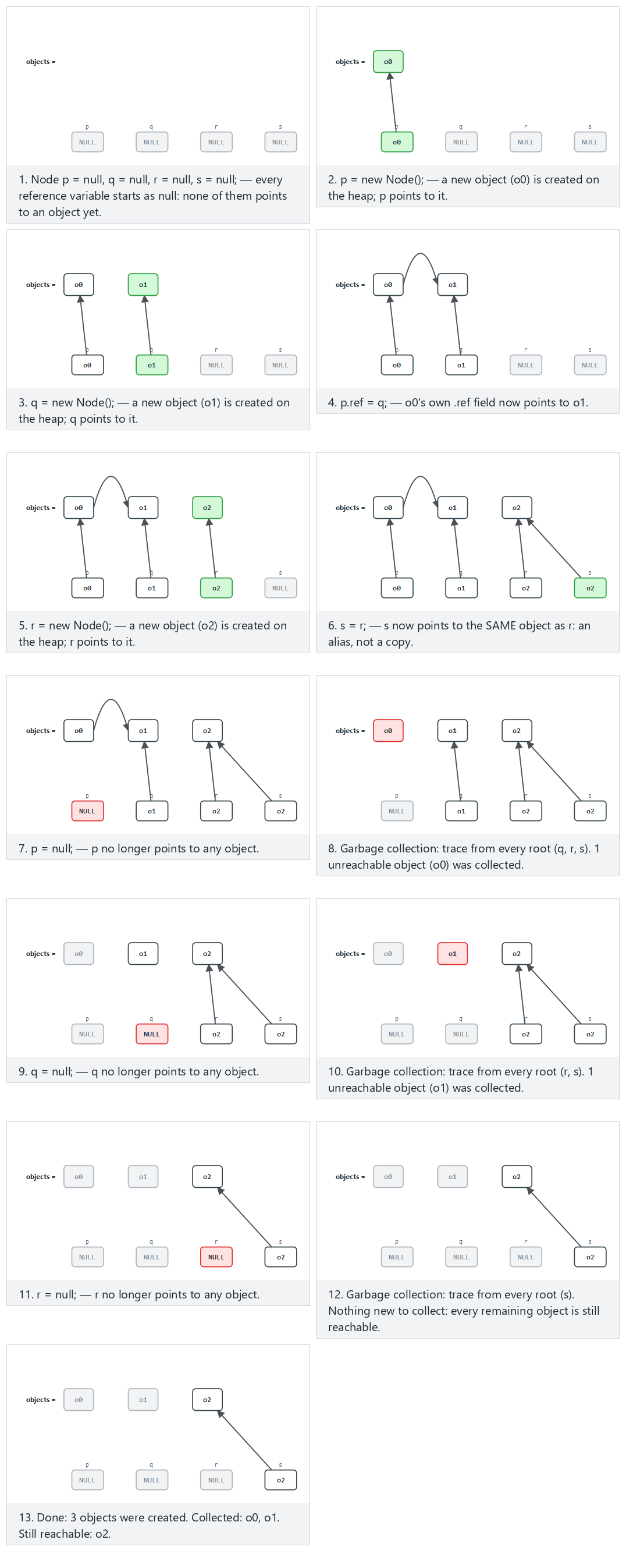
/* Week 1 -- Introduction to Data Structures
 * Two references can alias the same heap object; when no reference is left,
 * the object becomes eligible for garbage collection.
 * CEN207 Data Structures (CS50-style lecture notes)
 */
public class ReferenceAliasing {
    static class Counter {
        int value;
        Counter(int value) { this.value = value; }
    }

    public static void main(String[] args) {
        Counter a = new Counter(1);
        Counter b = a;              // b is an ALIAS: same object, not a copy

        System.out.println("a.value = " + a.value + ", b.value = " + b.value);
        System.out.println("a and b refer to the same object: " + (a == b));

        b.value = 99;                // changing through b is visible through a too
        System.out.println("after b.value = 99: a.value = " + a.value);

        a = null;                    // one reference gone; still reachable through b
        System.out.println("a = " + a + ", b.value = " + b.value);

        b = null;                    // last reference gone: now eligible for GC
        System.out.println("b = " + b + " (the Counter object has no reachable reference left)");
    }
}
/* Week 1 -- Introduction to Data Structures
 * C has no garbage collector: losing the only pointer to a block
 * without freeing it first is a memory leak.
 * CEN207 Data Structures (CS50-style lecture notes)
 */
#include <stdio.h>
#include <stdlib.h>

int main(void) {
    int *a = malloc(sizeof(int));
    *a = 1;
    printf("a = %p, *a = %d\n", (void *) a, *a);

    int *b = a;               /* b is an ALIAS: same block, not a copy */
    printf("a and b point to the same block: %s\n", (a == b) ? "true" : "false");

    *b = 99;                  /* writing through b is visible through a too */
    printf("after *b = 99: *a = %d\n", *a);

    /* Correct order: free the block through one of the aliases, THEN clear both. */
    free(a);
    a = NULL;
    b = NULL;                 /* free() does not clear pointers for you -- we must */
    printf("freed and cleared: a = %p, b = %p\n", (void *) a, (void *) b);

    /* If we had instead run  a = NULL; b = NULL;  BEFORE calling free, the block
     * would still be sitting allocated with no pointer left to reach it -- a
     * memory leak. C never reclaims it on its own; only free() does. */

    return 0;
}
Try it
Expected output:
Both programs alias two names to one piece of memory and mutate it through one of the names. The difference is entirely in what happens at the end: the C program must free the block and clear every alias by hand — miss either step and you have a bug (a leak if you forget free, a dangling pointer if you clear/reuse an alias without freeing first). The Java program does neither: once b = null; removes the last reference, the object simply becomes collectible, and the collector — not the programmer — decides when to actually reclaim it. Java trades a little control (you cannot force an exact reclaim moment, and System.gc() is only ever a hint, never a command) for an entire category of bug becoming structurally impossible.
Common mistakes
- Using a pointer after
freeing it (a dangling pointer) instead of setting it toNULLimmediately after freeing. Reading or writing through it is undefined behavior — it might silently corrupt unrelated memory long before your program visibly misbehaves. - Calling
freetwice on the same pointer (a double free) — corrupts the allocator's own bookkeeping. Setting the pointer toNULLafter freeing also makes this safe:free(NULL)is explicitly guaranteed to do nothing. - Forgetting
freeon a path your function returns early from (for example, inside anifbefore the normal end of the function) — a memory leak that only shows up after the program has been running a long time. - Assuming Java's GC means memory problems are impossible. Objects you keep an unnecessary reference to (for example, in a collection you forgot to clear) cannot be collected and still leak, in effect — the mechanism is different, the mistake is the same idea: something still points to data you no longer need.
Test yourself: stack, heap, and memory management
1. A function declares int arr[100]; as a local variable and returns a pointer to it. What is wrong?
arr lives on the stack, in that function's frame. The moment the function returns, its frame is popped and arr's memory is no longer valid — the returned pointer is already dangling before the caller even uses it. (The fix: allocate with malloc instead, so the memory survives the function returning.)
2. Why does free(block); block = NULL; (in that order) matter, and what would go wrong with block = NULL; free(block);?
free needs the actual address to give back; if you NULL it first, free(NULL) does nothing and the block is never returned to the heap — a memory leak, and the original address is now lost forever (nothing points to it any more).
3. Why can a dangling pointer never occur in Java the way it does in C?
Java has no free: an object is only reclaimed once the garbage collector proves nothing can reach it, so there is never a moment where a reachable reference points at memory that has already been taken back.
5.7 Preview: array layout vs linked layout
One more contrast, previewing next week. An array reserves one contiguous block, so arr[i] is a single calculation — O(1). A linked list, which you will build starting next week, stores each value in its own individually allocated node, connected only by pointers.
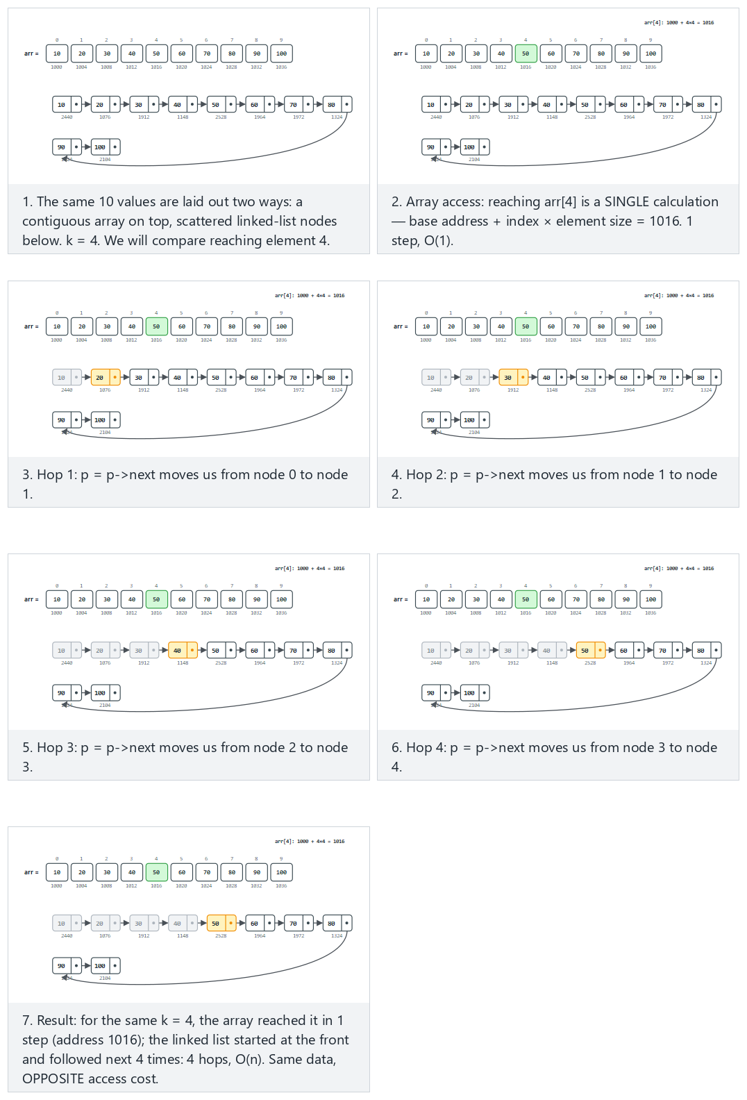
/* Week 1 -- Introduction to Data Structures
 * Preview of Week 2: five values laid out as a contiguous array
 * versus the same five values as individually allocated linked nodes.
 * CEN207 Data Structures (CS50-style lecture notes)
 */
#include <stdio.h>
#include <stdlib.h>

typedef struct Node {
    int data;
    struct Node *next;
} Node;

int main(void) {
    int arr[5] = {10, 20, 30, 40, 50};

    printf("array (contiguous):\n");
    for (int i = 0; i < 5; i++)
        printf("  arr[%d] = %d at %p\n", i, arr[i], (void *) &arr[i]);

    Node *head = NULL;
    for (int i = 4; i >= 0; i--) {
        Node *n = malloc(sizeof(Node));
        n->data = arr[i];
        n->next = head;
        head = n;
    }

    printf("\nlinked list (scattered, connected by pointers):\n");
    for (Node *n = head; n != NULL; n = n->next)
        printf("  node at %p: data = %d, next = %p\n", (void *) n, n->data, (void *) n->next);

    for (Node *n = head; n != NULL;) {
        Node *tmp = n;
        n = n->next;
        free(tmp);
    }

    return 0;
}
/* Week 1 -- Introduction to Data Structures
 * Preview of Week 2: the same five values as a contiguous array
 * versus a chain of individually created linked nodes.
 * CEN207 Data Structures (CS50-style lecture notes)
 */
public class ArrayVsLinkedPreview {
    static class Node {
        int data;
        Node next;
        Node(int data, Node next) { this.data = data; this.next = next; }
    }

    public static void main(String[] args) {
        int[] arr = {10, 20, 30, 40, 50};

        System.out.println("array (one contiguous block, indexed access):");
        for (int i = 0; i < arr.length; i++)
            System.out.println("  arr[" + i + "] = " + arr[i]);

        Node head = null;
        for (int i = arr.length - 1; i >= 0; i--)
            head = new Node(arr[i], head);

        System.out.println();
        System.out.println("linked list (separate objects, followed one .next at a time):");
        for (Node n = head; n != null; n = n.next)
            System.out.println("  node@" + Integer.toHexString(System.identityHashCode(n))
                    + ": data = " + n.data);
    }
}
Full program: array_vs_linked_preview.c / ArrayVsLinkedPreview.java
/* Week 1 -- Introduction to Data Structures
 * Preview of Week 2: the same values laid out as a contiguous array versus individually
 * allocated linked nodes; compare reaching element k: 1 step in the array vs k hops in the list.
 * Runs the same normal / hard / edge-case scenarios as the array-vs-linked-preview animation.
 * Real addresses are printed (yours will differ) -- only the array's fixed 4-byte stride and the
 * "1 step vs k hops" access-cost story are guaranteed to match.
 * CEN207 Data Structures (CS50-style lecture notes)
 */
#include <stdio.h>
#include <stdlib.h>

typedef struct Node {
    int data;
    struct Node *next;
} Node;

static void run_scenario(const char *label, const int values[], int n, int k) {
    printf("-- %s (k = %d) --\n", label, k);

    int arr[64];
    for (int i = 0; i < n; i++) arr[i] = values[i];

    printf("array (contiguous):\n");
    for (int i = 0; i < n; i++)
        printf("  arr[%d] = %d at %p\n", i, arr[i], (void *) &arr[i]);
    printf("array access: arr[%d] = %d, ONE calculation (base + %d*4). O(1).\n", k, arr[k], k);

    Node *head = NULL;
    for (int i = n - 1; i >= 0; i--) {
        Node *node = malloc(sizeof(Node));
        node->data = arr[i];
        node->next = head;
        head = node;
    }

    printf("linked list (scattered, connected by pointers):\n");
    for (Node *p = head; p != NULL; p = p->next)
        printf("  node at %p: data = %d, next = %p\n", (void *) p, p->data, (void *) p->next);

    Node *reached = head;
    int hops = 0;
    for (int h = 0; h < k; h++) { reached = reached->next; hops++; }
    printf("linked access: reached node with data = %d after %d hop%s. O(n).\n\n",
           reached->data, hops, hops == 1 ? "" : "s");

    for (Node *n2 = head; n2 != NULL;) {
        Node *tmp = n2;
        n2 = n2->next;
        free(tmp);
    }
}

int main(void) {
    /* normal: 10 values, k = 4 (in the middle) */
    int normal[] = {10, 20, 30, 40, 50, 60, 70, 80, 90, 100};
    run_scenario("normal: 10 values, k = 4 (in the middle)", normal, 10, 4);

    /* hard: 16 values, k = 13 (near the end) */
    int hard[] = {11, 22, 33, 44, 55, 66, 77, 88, 99, 111, 122, 133, 144, 155, 166, 177};
    run_scenario("hard: 16 values, k = 13 (near the end)", hard, 16, 13);

    /* edge: k = 0, the first element */
    int first[] = {7, 14, 21, 28, 35, 42, 49, 56, 63, 70};
    run_scenario("edge: k = 0, the first element", first, 10, 0);

    /* edge: k = the last index, the most hops */
    int last[] = {3, 6, 9, 12, 15, 18, 21, 24, 27, 30, 33, 36};
    run_scenario("edge: k = the last index, the most hops", last, 12, 11);

    return 0;
}
/* Week 1 -- Introduction to Data Structures
 * Preview of Week 2: the same values laid out as a contiguous array versus individually
 * created linked nodes; compare reaching element k: 1 step in the array vs k hops in the list.
 * Runs the same normal / hard / edge-case scenarios as the array-vs-linked-preview animation.
 * Java has no raw addresses, so per-object identity hashes stand in for "where it lives"
 * (yours will differ) -- only the "1 step vs k hops" access-cost story is guaranteed to match.
 * CEN207 Data Structures (CS50-style lecture notes)
 */
public class ArrayVsLinkedPreview {
    static class Node {
        int data;
        Node next;
        Node(int data, Node next) { this.data = data; this.next = next; }
    }

    static void runScenario(String label, int[] values, int k) {
        System.out.println("-- " + label + " (k = " + k + ") --");
        int n = values.length;

        System.out.println("array (one contiguous block, indexed access):");
        for (int i = 0; i < n; i++)
            System.out.println("  arr[" + i + "] = " + values[i]);
        System.out.println("array access: arr[" + k + "] = " + values[k] + ", ONE index computation. O(1).");

        Node head = null;
        for (int i = n - 1; i >= 0; i--)
            head = new Node(values[i], head);

        System.out.println("linked list (separate objects, followed one .next at a time):");
        for (Node p = head; p != null; p = p.next)
            System.out.println("  node@" + Integer.toHexString(System.identityHashCode(p)) + ": data = " + p.data);

        Node reached = head;
        int hops = 0;
        for (int h = 0; h < k; h++) { reached = reached.next; hops++; }
        System.out.println("linked access: reached node with data = " + reached.data + " after " + hops
                + " hop" + (hops == 1 ? "" : "s") + ". O(n).");
        System.out.println();
    }

    public static void main(String[] args) {
        // normal: 10 values, k = 4 (in the middle)
        int[] normal = {10, 20, 30, 40, 50, 60, 70, 80, 90, 100};
        runScenario("normal: 10 values, k = 4 (in the middle)", normal, 4);

        // hard: 16 values, k = 13 (near the end)
        int[] hard = {11, 22, 33, 44, 55, 66, 77, 88, 99, 111, 122, 133, 144, 155, 166, 177};
        runScenario("hard: 16 values, k = 13 (near the end)", hard, 13);

        // edge: k = 0, the first element
        int[] first = {7, 14, 21, 28, 35, 42, 49, 56, 63, 70};
        runScenario("edge: k = 0, the first element", first, 0);

        // edge: k = the last index, the most hops
        int[] last = {3, 6, 9, 12, 15, 18, 21, 24, 27, 30, 33, 36};
        runScenario("edge: k = the last index, the most hops", last, 11);
    }
}
Try it
Expected output (your addresses will differ):
array (contiguous):
  arr[0] = 10 at 000000A8783FF8A0
  arr[1] = 20 at 000000A8783FF8A4
  arr[2] = 30 at 000000A8783FF8A8
  arr[3] = 40 at 000000A8783FF8AC
  arr[4] = 50 at 000000A8783FF8B0

linked list (scattered, connected by pointers):
  node at 000001EEABFF34F0: data = 10, next = 000001EEABFF34D0
  node at 000001EEABFF34D0: data = 20, next = 000001EEABFF34B0
  node at 000001EEABFF34B0: data = 30, next = 000001EEABFF3490
  node at 000001EEABFF3490: data = 40, next = 000001EEABFF3470
  node at 000001EEABFF3470: data = 50, next = 0000000000000000
Expected output (the node@... identifiers are Java's per-object identity hashes, not real addresses, and will differ on your machine):
Notice the array addresses: ...8A0, ...8A4, ...8A8, ... — each exactly 4 bytes after the previous one, always, guaranteed by the language. The linked list's node addresses have no such guarantee at all; on this particular run they even happened to land close together, but nothing promises that — only the next pointers, drawn as arrows above, are guaranteed to connect the right values in the right order. Next week you will build, search, insert into and delete from exactly this structure.
6. ASN.1, BER TLV, and PER TLV: encoding data for the wire
6.1 A question to start
Two programs — maybe written in different languages, running on different machines, one big-endian and one little-endian — need to exchange a structured record (a name, an age, ...) as a stream of bytes. A struct in memory is not portable: its exact byte layout depends on the compiler, the platform, and padding rules. How do two completely different programs agree, byte for byte, on what a record looks like on the wire?
6.2 A short history
ASN.1 (Abstract Syntax Notation One) is an ITU-T/ISO standard for describing structured data independently of any programming language or machine. It originated as CCITT (now ITU-T) recommendation X.409 in 1984, as part of the X.400 messaging standards, and was split out and substantially revised as the X.680 series starting in 1995 — the version still in use today. BER (Basic Encoding Rules, X.690) is ASN.1's original, self-describing encoding: every value is tagged and length-prefixed, so a decoder can walk the bytes without knowing the schema in advance. PER (Packed Encoding Rules, X.691, 1994) came later, designed for bandwidth-constrained links: if both sides already know the schema, most of BER's tags and lengths are redundant and PER packs the bits far more tightly. ASN.1 with BER still underlies protocols you use constantly and invisibly — X.509 certificates (the basis of HTTPS), LDAP, and SNMP among them.
6.3 Intuition: an envelope with a label, a size, and the contents
The core idea behind BER is simple enough to do by hand: every value is wrapped in three parts, in order —
- Tag: what kind of value this is (an integer? a string? a whole record?)
- Length: how many bytes the value's content takes
- Value: the content itself, which — for a record made of several fields — is simply several more Tag-Length-Value groups back to back
This pattern is universally called TLV. A decoder that has never seen your specific record before can still walk it correctly: read a tag, read a length, skip (or interpret) exactly that many bytes, repeat.
6.4 The TLV byte layout
| Part | Size | What it encodes |
|---|---|---|
| Tag | 1 byte (for the small tag numbers used here) | 2 bits: class (universal/application/context/private) · 1 bit: primitive (0) or constructed (1, i.e. "contains more TLVs") · 5 bits: tag number |
| Length | 1 byte, short form (values 0-127) | The number of content bytes that follow. Values ≥ 128 need the long form: a first byte with its top bit set giving the count of following length bytes, then that many bytes of the actual length, big-endian |
| Value | Length bytes | The raw content — a number, a string, or (for a constructed type like SEQUENCE) more TLVs concatenated |
Two tags used below are real ASN.1 universal-class tag numbers: INTEGER is universal tag number 2 (0x02), UTF8String is tag number 12 (0x0C), and SEQUENCE — a constructed type holding an ordered list of other values — is tag number 16 with the constructed bit set (0x30).
6.5 Encoding a small record by hand
We will encode SEQUENCE { name: UTF8String "Rex", age: INTEGER 5 } — a two-field record — one byte group at a time.

/* Week 1 -- Introduction to Data Structures
 * Hand-encode a tiny record as BER TLV: SEQUENCE { name UTF8String, age INTEGER }.
 * CEN207 Data Structures (CS50-style lecture notes)
 */
#include <stdio.h>
#include <string.h>

#define TAG_INTEGER    0x02
#define TAG_UTF8STRING 0x0C
#define TAG_SEQUENCE   0x30   /* universal class, constructed, tag number 16 */

static int encode_tlv(unsigned char *out, unsigned char tag, const unsigned char *value, int len) {
    out[0] = tag;
    out[1] = (unsigned char) len;    /* short form: length < 128 fits in one byte */
    memcpy(out + 2, value, (size_t) len);
    return 2 + len;
}

static void print_bytes(const char *label, const unsigned char *buf, int len) {
    printf("%s (%d bytes):", label, len);
    for (int i = 0; i < len; i++)
        printf(" %02X", buf[i]);
    printf("\n");
}

int main(void) {
    unsigned char name_tlv[16], age_tlv[16], record[32], content[32];
    const unsigned char name_value[] = "Rex";
    unsigned char age_value = 5;

    int name_len = encode_tlv(name_tlv, TAG_UTF8STRING, name_value, 3);
    print_bytes("name TLV ", name_tlv, name_len);

    int age_len = encode_tlv(age_tlv, TAG_INTEGER, &age_value, 1);
    print_bytes("age TLV  ", age_tlv, age_len);

    memcpy(content, name_tlv, (size_t) name_len);
    memcpy(content + name_len, age_tlv, (size_t) age_len);
    int content_len = name_len + age_len;

    int record_len = encode_tlv(record, TAG_SEQUENCE, content, content_len);
    print_bytes("SEQUENCE ", record, record_len);

    return 0;
}
/* Week 1 -- Introduction to Data Structures
 * Hand-encode a tiny record as BER TLV: SEQUENCE { name UTF8String, age INTEGER }.
 * CEN207 Data Structures (CS50-style lecture notes)
 */
import java.io.ByteArrayOutputStream;
import java.nio.charset.StandardCharsets;

public class TlvEncoding {
    static final int TAG_INTEGER = 0x02;
    static final int TAG_UTF8STRING = 0x0C;
    static final int TAG_SEQUENCE = 0x30;   // universal class, constructed, tag number 16

    static byte[] encodeTlv(int tag, byte[] value) {
        ByteArrayOutputStream out = new ByteArrayOutputStream();
        out.write(tag);
        out.write(value.length);            // short form: length < 128 fits in one byte
        out.writeBytes(value);
        return out.toByteArray();
    }

    static String toHex(byte[] bytes) {
        StringBuilder sb = new StringBuilder();
        for (byte b : bytes)
            sb.append(String.format("%02X ", b));
        return sb.toString().trim();
    }

    public static void main(String[] args) {
        byte[] nameTlv = encodeTlv(TAG_UTF8STRING, "Rex".getBytes(StandardCharsets.UTF_8));
        System.out.println("name TLV  (" + nameTlv.length + " bytes): " + toHex(nameTlv));

        byte[] ageTlv = encodeTlv(TAG_INTEGER, new byte[] {5});
        System.out.println("age TLV   (" + ageTlv.length + " bytes): " + toHex(ageTlv));

        ByteArrayOutputStream content = new ByteArrayOutputStream();
        content.writeBytes(nameTlv);
        content.writeBytes(ageTlv);

        byte[] record = encodeTlv(TAG_SEQUENCE, content.toByteArray());
        System.out.println("SEQUENCE  (" + record.length + " bytes): " + toHex(record));
    }
}
Try it
Expected output:
Read the final 10 bytes as a decoder would, left to right, with no prior knowledge of the record's shape: 30 — a constructed, universal, tag-16 value (a SEQUENCE) — 08 — its content is the next 8 bytes — then, inside that content, 0C 03 52 65 78 (a UTF8String of length 3, "Rex") followed by 02 01 05 (an INTEGER of length 1, 5). Every byte has a job; nothing is guessed or assumed from context.
6.6 BER vs PER
| BER | PER | |
|---|---|---|
| Self-describing | Yes — every value carries its own tag and length | No — both sides must already agree on the schema |
| Size | Larger: at least 2 extra bytes (tag + length) per field | Much smaller: no tags, lengths only where the schema can't infer them, values packed bit by bit |
| Can a generic decoder read it without the schema? | Yes | No — the schema is required to decode at all |
| Typical use | X.509 certificates, LDAP, SNMP — interoperability across many independent implementations | Bandwidth-critical protocols (e.g. cellular signaling) where every byte on the wire matters |
Both encode the exact same abstract information (an ASN.1 schema, written once) — BER trades size for self-description, PER trades self-description for size. This course's example above is BER; PER is worth knowing exists, but hand-packing individual bits is outside this course's scope.
Common mistakes
- Forgetting the length prefix and hoping a fixed-size read on the other end will "just work". TLV exists specifically so the reader never has to guess a size.
- Assuming length always fits in one byte. The short form used here only works for lengths under 128; real BER decoders must also handle the long form for anything bigger.
- Mixing up
Length(the number of content bytes, i.e. theVin TLV) with the size of the whole TLV (Tag+Lengthbytes + content) — the SEQUENCE example above hasLength = 8but the whole encoded SEQUENCE is 10 bytes. - Treating BER and PER as interchangeable on the wire. They are two different byte formats for the same schema; a PER decoder cannot parse BER bytes, or vice versa.
Test yourself: ASN.1 and TLV
1. What do the three letters in TLV stand for, and in what order do they appear on the wire?
Tag, Length, Value — in exactly that order: first what kind of thing this is, then how many bytes it takes, then the bytes themselves.
2. Why is SEQUENCE's tag byte 0x30 and not 0x10 (tag number 16 in binary, 10000)?
Because the top three bits of the tag byte are not part of the tag number: two class bits (00 for universal) and one constructed bit, which is 1 here because a SEQUENCE contains other TLVs. 00 1 10000 = 0x30.
3. Why does PER need the schema to decode, while BER does not?
PER drops the tag and (where possible) the length to save space, so a PER decoder can only tell where one field ends and the next begins if it already knows, from the schema, each field's type and, where relevant, its size.
7. Hands-on lab: the C toolchain
7.1 Why this matters
Every idea in this course is worthless to you until it compiles and runs. From this point on, every week hands you C and Java programs and asks you to build and run them yourself — and the midterm project (see the project guide) is graded, in part, on whether it builds cleanly with CMake on a fresh clone. This lab sets up, once, the exact workflow you will repeat all semester: compile, run, debug, plus the build tool (CMake) the project template uses.
7.2 The toolchain, briefly
A C compiler translates your source file into machine code; a linker (often invoked as part of the same gcc command) stitches your code together with the C standard library into one executable. GCC, the GNU Compiler Collection, was started by Richard Stallman in 1987 as part of the GNU project and remains one of the two compilers you are most likely to use in this course (the other being Microsoft's MSVC, inside Visual Studio, on Windows). GDB, the GNU Debugger, dates to the same GNU project, 1986, and lets you pause a running program, inspect its variables, and step through it line by line — exactly what Section 7.5 does below. CMake is a build-system generator: you describe what to build in a CMakeLists.txt, and CMake produces the actual build files for whatever tool you have installed (Makefiles, Ninja, a Visual Studio solution, ...) — this is why the same project builds on Windows, WSL, and Linux without three separate sets of instructions.
7.3 Step 1: your first compile and run
Every program in this course, from here on, is built and run the same way. Start with the simplest possible one.
Try it
Expected output:
Three things happened: gcc compiled hello_workshop.c into an executable named x (-o /tmp/x); && then ran that executable only if the compile succeeded (a compile error produces no executable, and there is nothing to run); the program printed one line and exited.
7.4 Step 2: compile with warnings on, and read them
-Wall -Wextra turns on a wide set of warnings that a bare gcc file.c stays silent about — unused variables, suspicious comparisons, format-string mismatches, and more. Every program in this course, including your project, must compile without warnings under these flags: a warning is the compiler telling you something is probably a bug, before you find out the hard way at runtime. Try it yourself: change printf("%d\n", n) in any program to printf("%s\n", n) (wrong format specifier for an int) and recompile with -Wall -Wextra — gcc will point at the exact line and tell you the format string does not match the argument. Fix the mismatch before moving on, every time; never "fix" a warning by silencing it.
7.5 Step 3: find a bug with gdb
Here is a small program with a genuine bug: the average it prints is wrong.
/* Week 1 -- Introduction to Data Structures
 * A small bug hunt for the C workshop: why is the average wrong?
 * CEN207 Data Structures (CS50-style lecture notes)
 */
#include <stdio.h>

int average_buggy(const int arr[], int n) {
    int sum = 0;
    for (int i = 0; i < n; i++)
        sum = sum + arr[i];
    return sum / n;               /* bug: integer division truncates */
}

double average_fixed(const int arr[], int n) {
    int sum = 0;
    for (int i = 0; i < n; i++)
        sum = sum + arr[i];
    return (double) sum / n;      /* fix: promote to double before dividing */
}

int main(void) {
    int scores[] = {7, 8, 8};
    int n = (int) (sizeof(scores) / sizeof(scores[0]));

    printf("average_buggy  -> %d\n", average_buggy(scores, n));
    printf("average_fixed  -> %.2f\n", average_fixed(scores, n));

    return 0;
}
Build it with debug symbols (-g), so gdb can show source lines and variable names instead of raw addresses:
Inside the (gdb) prompt, type these commands one at a time (each (gdb) line below is something you type; everything else is gdb's response):
(gdb) break debug_average.c:11
(gdb) run
(gdb) print sum
(gdb) print n
(gdb) print sum / n
(gdb) print (double) sum / n
(gdb) continue
(gdb) quit
Expected session (a couple of gdb's own thread-lifecycle lines are trimmed for clarity; everything else is exactly what gdb prints):
Breakpoint 1 at 0x140001768: file debug_average.c, line 11.

Thread 1 hit Breakpoint 1, average_buggy (arr=0x5ffe80, n=3) at debug_average.c:11
11          return sum / n;               /* bug: integer division truncates */
$1 = 23
$2 = 3
$3 = 7
$4 = 7.666666666666667
average_buggy  -> 7
average_fixed  -> 7.67
Walk through what just happened: break debug_average.c:11 set a breakpoint on the return line inside average_buggy; run started the program, which stopped exactly there, before that line executed. print sum and print n showed the real values at that point (23 and 3 — correct so far: 7 + 8 + 8 = 23). print sum / n showed 7 — integer division, which truncates 23 / 3 = 7.666... down to 7. print (double) sum / n showed the intended result, 7.666666666666667, by forcing floating-point division. The bug was never in the loop or the sum — it was the final division. average_fixed (Section-visible in the code above) fixes it with exactly that cast, and its %.2f output, 7.67, matches. This — form a hypothesis, inspect a variable, confirm or refute it — is the entire method of debugging with a debugger, and it scales to bugs far subtler than this one.
7.6 Step 4: CMake basics
The midterm project template (see the project guide) is built with CMake, not a bare gcc command. A CMakeLists.txt describes what to build; CMake figures out how, for whatever platform you are on.
cmake_minimum_required(VERSION 3.20)
project(week1_cmake_demo C)

add_executable(week1_cmake_demo main.c)
/* Week 1 -- Introduction to Data Structures
 * The program built by the CMake basics demo in the C workshop.
 * CEN207 Data Structures (CS50-style lecture notes)
 */
#include <stdio.h>

int main(void) {
    printf("Built with CMake: week1_cmake_demo\n");
    return 0;
}
Try it (run from inside the cmake-demo folder, which holds both files above):
Expected output:
-- The C compiler identification is GNU 13.1.0
-- Detecting C compiler ABI info
-- Detecting C compiler ABI info - done
-- Check for working C compiler: C:/Strawberry/c/bin/gcc.exe - skipped
-- Detecting C compile features
-- Detecting C compile features - done
-- Configuring done (1.8s)
-- Generating done (0.0s)
-- Build files have been written to: <your build folder>

[ 50%] Building C object CMakeFiles/week1_cmake_demo.dir/main.c.obj
[100%] Linking C executable week1_cmake_demo.exe
[100%] Built target week1_cmake_demo

Built with CMake: week1_cmake_demo
cmake -S . -B build configures the project: it reads CMakeLists.txt, checks the compiler works, and writes build files into a new build/ folder (never commit this folder to Git — the project's .gitignore should already exclude it). cmake --build build actually compiles and links, calling whatever underlying tool was generated (here, mingw32-make). The -G "MinGW Makefiles" flag pins the generator to match the gcc used throughout this course; leaving it out lets CMake pick a sensible default for your system (Unix Makefiles on Linux/WSL, a Visual Studio solution on Windows) — both are fine, and the prerequisites page has the exact setup for each.
7.7 A note on Visual Studio
Everything above has a menu-driven equivalent in Visual Studio, which many of you will use on Windows: Build → Build Solution compiles (equivalent to gcc/cmake --build); Debug → Start Debugging (F5) runs under the debugger; clicking in the left margin of the editor sets a breakpoint (equivalent to gdb's break); once stopped, the Locals/Watch panes show variable values (equivalent to gdb's print), and Debug → Step Over/Step Into (F10/F11) step through code line by line. Visual Studio can also open a CMakeLists.txt directly ("Open a local folder") and will configure and build it without a separate .sln file — the same CMakeLists.txt from Section 7.6 works unchanged.
Common mistakes
- Forgetting
-std=c11(or building with an editor's default, which may be an older or newer standard) and getting different behavior than a classmate on a different setup. Always pin the standard explicitly, as every "Try it" block in this course does. - Committing a
build/folder (or.o/.obj/.exefiles) to Git. These are generated from source and belong in.gitignore, not in version control. - Running a stale executable after a compile that actually failed, and being confused why your "fix" had no effect — always check the compiler's exit status, or simply chain the run with
&&as every example in these notes does. - Reaching for
printfdebugging (adding print statements everywhere) as the only tool, when a two-minute gdb session — set a breakpoint, print a few variables — answers the same question with no code changes to remove afterward.
Test yourself: the C workshop
1. What does -Wall -Wextra do, and why does this course require code to compile cleanly under it?
It enables a wide set of compiler warnings beyond the bare minimum. Warnings usually point at real bugs (mismatched types, unused variables, suspicious comparisons); requiring a clean build means those bugs get fixed immediately, not discovered later at runtime.
2. In the gdb session above, why did print sum / n and print (double) sum / n give different answers for the same sum and n?
sum and n are both int, so sum / n performs integer division and truncates toward zero (23 / 3 = 7). Casting to double first forces floating-point division, giving the true value (7.666...). Same variables, different arithmetic.
3. What is the difference between what cmake -S . -B build does and what cmake --build build does?
The first configures: it reads CMakeLists.txt and generates build files for your platform's tool, without compiling anything. The second builds: it invokes that generated tool to actually compile and link the program.
Summary
| Idea | Key fact |
|---|---|
| Data structure | A way of organizing data so specific operations have a known, analyzable cost — there is no single best structure, only trade-offs |
| Linear vs non-linear | Linear: every element has one "next" (arrays, lists, stacks, queues). Non-linear: an element can have several (trees, graphs) |
| Big-O | An upper bound on how cost grows with n, ignoring constants — read off the dominant term |
| Best / worst / average case | The same algorithm can take a different number of steps depending on which input it gets, not just how big it is |
| Space complexity | The same counting idea, applied to extra memory instead of steps |
| Pointer (C) | A variable that stores an address; & takes an address, * follows one, -> follows-then-accesses-a-field |
| Reference (Java) | The same "points to shared data" idea, with no raw addresses, no arithmetic, and automatic safety |
| Stack (memory region) | One frame per active call, LIFO, freed automatically — fast, but limited in size and lifetime |
| Heap | Explicitly requested (malloc/new) and, in C, explicitly released (free); in Java, reclaimed automatically by the garbage collector |
| TLV / ASN.1 BER | Tag + Length + Value, recursively — a self-describing way to put structured data on the wire |
| C toolchain | Compile with gcc -std=c11 -Wall -Wextra, debug with gdb, build multi-file projects with CMake |
| Algorithm | Complexity | Needs |
|---|---|---|
| Linear search | O(n) worst case, O(1) best case | Nothing — works on any array |
| Binary search | O(log n) worst case | A sorted array |
Exercises
- Add a
peek(int i)-style thought experiment: for an array ofnelements, what is the Big-O of reading the element at indexidirectly (arr[i]), and why does that not depend oniorn? - Modify
linear_search(Section 3.4) so it counts comparisons and returns the number of comparisons the first occurrence of a repeated value took, given an array that may contain duplicates. - Using the pointer rules from Section 4.4, write (on paper first) a
swap(int *a, int *b)function in C that actually exchanges the values of twointvariables in the caller — the problem posed in Section 4.1. Then explain in one sentence why the equivalent is not directly possible for twointvariables in Java. - Extend
stack_vs_heap.c(Section 5.5) with a second heap block, allocated after the first is freed. Predict, before running it, whether the new block's address will reuse the freed one's address on your system — then run it and check. - Hand-encode
SEQUENCE { flag: BOOLEAN true, count: INTEGER 200 }as BER TLV bytes on paper. (Hint:BOOLEANis universal tag number 1;TRUEis conventionally encoded as the single byte0xFF.200does not fit in one signed byte — you will need two content bytes,0x00 0xC8, so the leading bit is not mistaken for a sign bit.)
Exercise answers (sketch)
- O(1).
arr[i]computesbase_address + i * element_size— one multiplication and one addition, always, regardless ofnori. - Keep the existing comparison counter unchanged (it already stops at the first match via
return i;); the function already answers this — the exercise is realizing no change is needed, only recognizing why. void swap(int *a, int *b) { int t = *a; *a = *b; *b = t; }, called asswap(&x, &y);. Java has no&/*for primitiveintvariables — a Java method only ever receives a copy of anintargument, so there is no way to reach back into the caller's variable at all; the same trick works in Java only for objects/arrays, because those parameters already carry a reference to shared data.- Answers vary by system and allocator; many small allocators do reuse a just-freed block of the same size for the next request of the same size, but this is never guaranteed by the C standard — treat it as an implementation detail, never as something your program may rely on.
BOOLEAN: tag0x01, length0x01, value0xFF→01 01 FF.INTEGER 200: tag0x02, length0x02, value00 C8→02 02 00 C8. Wrapped in aSEQUENCE: content =01 01 FF 02 02 00 C8(7 bytes), so the full encoding is30 07 01 01 FF 02 02 00 C8(9 bytes total).
Self-check quiz
1. Why can two different algorithms both be correct but have very different Big-O?
Big-O measures how the number of steps grows with input size, not whether the answer is right. Two correct algorithms can reach the same answer through very different amounts of work — linear search and binary search both correctly find a value, at O(n) and O(log n) respectively.
2. Put these in order from fastest- to slowest-growing: O(n log n), O(1), O(n), O(log n), O(n²).
O(1) < O(log n) < O(n) < O(n log n) < O(n²).
3. Why does binary search require a sorted array but linear search does not?
Binary search decides which half to discard by comparing the target to the middle element — that comparison only tells you anything useful if everything to one side is guaranteed smaller and everything to the other side is guaranteed larger, which is exactly what "sorted" means. Linear search never relies on any ordering; it just checks every element.
4. What does int *p mean, and what is the difference between p and *p?
p is declared as a pointer to an int — a variable that stores the address of an int. p (used later, not in the declaration) is that address; *p dereferences it, meaning "the int value stored at that address."
5. Why does p->x exist as a shorthand, and what is it shorthand for?
p->x is shorthand for (*p).x: dereference the pointer p to reach the struct it points to, then access its x field. It exists because this combination (pointer to a struct, then a field access) is extremely common in C code.
6. A local array declared inside a function is on the stack. What happens to it the instant the function returns?
Its stack frame is popped and the memory is no longer valid — any pointer to it becomes dangling immediately. This is why a function must never return the address of one of its own local (non-static) variables.
7. In C, what two things must you do, together, to avoid a dangling pointer after you no longer need a heap block?
Call free() on the pointer to release the block back to the heap, and then set the pointer itself to NULL so it can never accidentally be dereferenced afterward.
8. Why is it structurally impossible to have a dangling pointer in Java?
Java has no free. The garbage collector only reclaims an object once it has proven nothing in the program can reach it any more — so there is never a reachable reference pointing at memory that has already been taken back.
9. In a BER TLV encoding, what does the Length field actually count?
The number of bytes in the Value that immediately follows it — not the size of the Tag or Length bytes themselves, and not the size of the whole TLV group.
10. What is the one command that turns a CMakeLists.txt into an actual compiled program, after cmake -S . -B build has already been run once?
cmake --build build — it invokes the underlying build tool (Makefiles, Ninja, MSBuild, ...) that the configure step generated.
Looking ahead
Today built the two foundations every later week leans on: a way to measure cost (Big-O) and a picture of memory (pointers, stack, heap) precise enough to reason about. Next week puts both to immediate use: you will build a linked list — a chain of individually allocated nodes connected by exactly the kind of pointers you met in Section 4, living on exactly the heap you met in Section 5 — and see the O(1)-insert-anywhere, O(n)-access trade-off from Section 5.7's preview in full, with insertion, deletion, and traversal all written out and measured. From there, Week 3 puts a linked list under a very specific set of rules and calls the result a stack or a queue; Week 4 breaks the "one next" rule of linear structures on purpose and calls the result a tree; and every single one of those structures will be judged, from day one, with the same tool you built today: count the steps, name the O.
References
- Course syllabus, Week 1:
CEN207-2026-2027-Guz-Izlence.en.md. - D. E. Knuth. The Art of Computer Programming, Volume 1: Fundamental Algorithms, 3rd ed. Addison-Wesley, 1997 (1st ed. 1968) — the foundational treatment of data structures and their analysis.
- B. Liskov, S. Zilles. "Programming with Abstract Data Types." ACM SIGPLAN Notices, 1974 — the abstract data type distinction used throughout this course.
- D. E. Knuth. "Big Omicron and Big Omega and Big Theta." ACM SIGACT News, 8(2), 1976 — the article that standardized O/Ω/Θ notation for algorithm analysis in computer science.
- T. H. Cormen, C. E. Leiserson, R. L. Rivest, C. Stein. Introduction to Algorithms, 3rd ed. MIT Press — asymptotic notation, and searching algorithms.
- R. Sedgewick, K. Wayne. Algorithms, 4th ed. Addison-Wesley, 2011 — algorithm analysis and binary search.
- B. W. Kernighan, D. M. Ritchie. The C Programming Language, 2nd ed. Prentice Hall, 1988 — pointers,
struct, and memory management in C, from the language's own authors. - Y. Daniel Liang. Introduction to Java Programming, Comprehensive Version, 10th ed. — Java references and memory management.
- ITU-T Recommendation X.680 (ASN.1 syntax), X.690 (BER, CER, DER), and X.691 (PER) — the current ASN.1 encoding standards.
- GNU Project — GCC (GNU Compiler Collection) and GDB (GNU Debugger) documentation, gnu.org.
- Kitware — CMake documentation, cmake.org.